The Recommender's Lesson: How Scalable Learning Augments Human Insights

Introduction: A Story Told by the Bitter Lesson #

The journey of recommender systems is a quintessential case study of Rich Sutton's "The Bitter Lesson" in action^[1]. The essay posits that the greatest long-term gains in AI have consistently start with elaborate, human-designed knowledge but end with general-purpose methods that leverage massive increases in computation. The history of recommendation algorithms, from its origins in the 1990s to the generative foundation models today, is a powerful, domain-specific illustration of this principle.

The recommender systems, began as tools for managing information overload (Tapestry in 1992 from Xerox PARC^[2]), have become a cornerstone of the modern internet, serving billions of users daily^[3]. The core problem of understanding/predicting user preference has remained stable, but the methods for solving it have undergone multiple seismic shifts. This evolution can be understood as a progression through three distinct eras, each marking a step further away from human-curated systems and closer to scalable, computation-driven learning:

1. The Classical Era: Dominated by collaborative filtering (CF), matrix factorization (MF), and simple learning algorithms (logistic regression and tree-based models), these early models were elegant and effective but limited by their reliance on the user-item interaction matrix alone for CF and MF, or by low-order relationships between different features beyond the interaction matrix in simple learning algorithms. Further, they rely on intensive feature engineering.
2. The Deep Learning Era: Marked by the adoption of neural networks, this era began the process of automating feature learning, letting computation discover the complex, nonlinear relationships that humans previously had to engineer by hand. It also saw the rise of sequential modeling to capture the dynamic nature of user interests. Overall, it is a transition to simplify feature engineering and also shifting to neural networks as the main model with various architectures for different domains.
3. The Generative Era: The current frontier, inspired by the success of generative AI, especially Large Language Models (LLMs) for natural language processing (NLP), represents the lesson's latest expression^[3]. It seeks to replace the entire complex, multi-stage pipeline (a system composed of numerous specialized, human-designed components) with a single, massive, scalable learning machine that learns from raw data, paving the way for unified foundation models.

Core Recommendation Algorithms Evolution Overview #

Before dive into the details of each era, let's take a quick overview of the algorithmic evolution as depicted in Figure 1.

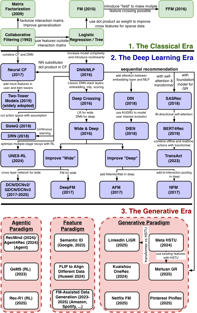
In the Classical Era, the recommendation algorithms can be traced back to the Collaborative Filtering (CF) and Logistic Regression (LR) model.

From CF, the Matrix Factorization (MF) method emerged to derive the user matrix and item matrix from the user-item interaction matrix. With user and item representation in latent vectors (a.k.a. embeddings), MF can handle data sparsity better and is more generalizable, but still limited by only using user-item interaction matrix. Later, the Neural Collaborative Filtering (NeuralCF) algorithm supported adding user and item signals to derive embeddings, and evolved into the famous two-tower models that is widely used across the industry.

The LR model provided a way to leverage more features than user-item interaction matrix before deep learning era. From the simple LR model, two major model evolution branches emerged in the Classical Era and Deep Learning Era, respectively.

The Factorization Machine Branch within the Classical Era: Recognizing the importance of feature interactions, LR evolved into the Factorization Machine (FM), which added a term to model all pairwise feature interactions efficiently via latent vectors. This line of work was further refined into Field-aware Factorization Machines (FFM), which allowed for more nuanced interactions by learning different latent vectors for each feature field.

The Deep Learning Era: The DL revolution extended LR's linear transformation into the nonlinear realm with DNNs/MLPs. In addition to the two-tower models evolution with neuralCF, the DL revolution has led to the following three branches of development:

1. Wide & Deep Architecture: Early pure-DNN models like Deep Crossing demonstrated the power of learning high-order feature interactions automatically with classic stack (embedding + MLP + output scoring). This led to the influential Wide & Deep architecture, which explicitly combined the strengths of a simple linear model (the "wide" part, a direct descendant of LR) for memorization and a DNN (the "deep" part) for generalization. The success of Wide & Deep spurred further innovation aimed at improving its components:
   • Improving the "Wide" Part: Models like Deep & Cross Network (DCN) and its variants and DeepFM replaced the manual feature engineering of the wide component with automated methods for learning feature interactions, drawing inspiration from the FM branch.
   • Improving the "Deep" Part: Concurrently, models like Neural Factorization Machines (NFM) and Attentional Factorization Machines (AFM) evolved from the FM branch to better model feature interactions within the deep learning paradigm itself, enhancing the "deep" component's ability to capture complex relationships.
2. The Sequential Modeling Branch: Building on the foundational concepts of embeddings and MLPs from the deep learning branch, a parallel evolution focused on modeling the sequence of user actions. This began with models like the Deep Interest Network (DIN) and the Transformer-based SASRec, which used attention mechanisms to capture dynamic user interests. This was further advanced by models like DIEN, which explicitly modeled the evolution of interests, and sophisticated industrial models like Pinterest's TransAct, which apply these principles at massive scale.
3. Reinforcement Learning and Bandits: This branch explores recommendation as a sequential decision process, focusing on the exploration-exploitation tradeoff. Early applications involved contextual multi-armed bandit algorithms (like LinUCB or Thompson Sampling) to adapt to real-time user feedback, as seen in Yahoo!'s news recommender. Later, full reinforcement learning formulations treated recommendation as a Markov Decision Process, aiming to optimize long-term user engagement, with examples like Slate-Q for selecting optimal slates of items. While full RL deployments remain complex, the concept of "value-aware recommendations" (optimizing for long-term metrics like lifetime value or retention) is gaining traction, with platforms like UNEX-RL for multi-stage RL optimization.

Figure 1 also summarizes the three major paradigms in the Generative Era that illustrate how foundation models empower recommender system development at scale, namely feature paradigm, generative paradigm, and agentic paradigm.

The Classical Era: From Collaborative Filtering to Matrix Factorization and Simple Learning with Manual and Explicit Feature Engineering #

The first fifteen years of recommender systems were defined by the development of foundational algorithms that established the core principles of personalization. This era moved from simple neighborhood-based heuristics to more powerful latent factor models.

Classical Recommendation Model Evolution #

Collaborative Filtering (CF) was the inaugural paradigm. Its premise is that the best recommendations come from people with similar tastes or similar items the target user has engaged before. Figure 2 illustrates the process for collaborative filter based on the user-item co-occurrence matrix (also known as interaction matrix), in which a user is represented by one row, an item is represented by one column, and each element in the matrix represents user-item interaction (rating, views, etc.). The collaborative filtering process can be implemented in two primary ways as detailed below.

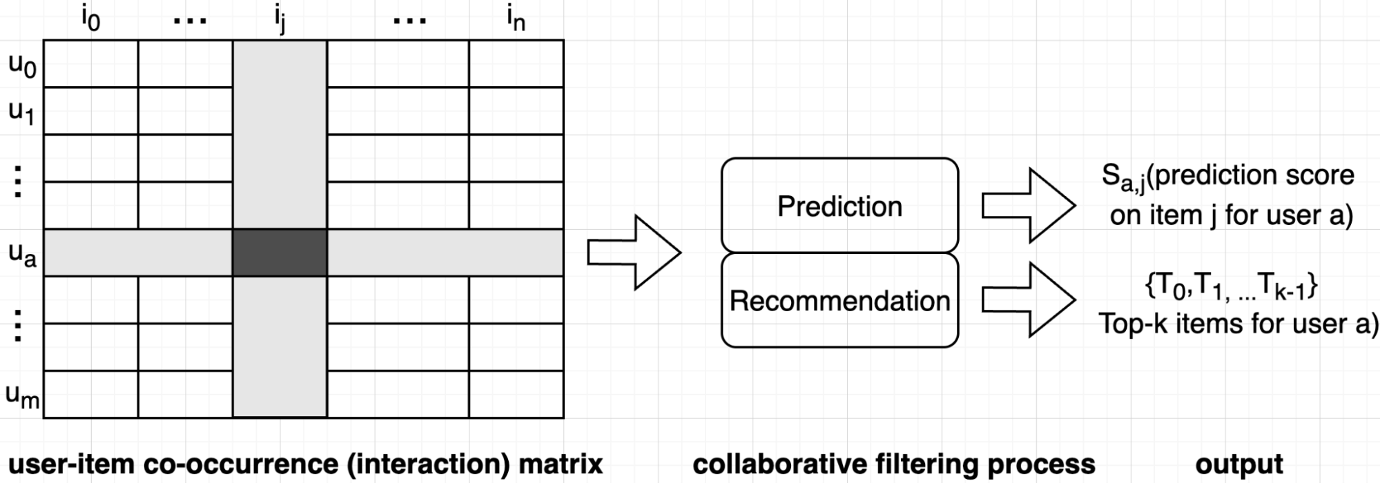
• User-based CF: To predict a user's rating for an item, the system finds other users with similar rating histories and calculates a weighted average of their ratings for that item.

  User similarity is defined by the similarity of user vectors, and many different similarity measures (such as cosine similarity, pearson similarity) can be used. Subsequently, we can generate the item recommendation based on the item scores given by top-n similar users to the target user like in Equation (1)

  $$S_{a,j}=\frac{\sum_{b \in B}{W_{a,b}S_{b,j}}}{\sum_{b \in B}{W_{a,b}}} \tag{1}$$

  where $B$ is the chosen user set that is similar to target user $a$ based on a similarity threshold, weight $W_{a,b}$ represents the similarity between user $a$ and $b$, $S_{b,j}$ is the score by user b for item j. While user-based CF is intuitive, it is not widely used since user history is sparse (hard to find similar users) and larger number of users at internet scale (co-occurance matrix grow proprotinally to the square of user number).

• Item-based CF: This approach, famously pioneered and scaled by Amazon.com in 2003, instead computes similarities between items based on user interaction patterns^[4],^[5]. For example, if users who buy item X also tend to buy item Y, the two items are considered similar. The key innovation was its scalability. By pre-computing an item-item similarity matrix offline, the system could generate real-time recommendations through a series of simple, fast lookups. This made it feasible for Amazon's massive catalog and customer base, representing a landmark in industrial recommender systems^[6]. In ItemCF, the item recommendation score for the target user is derived with Equation (2)

  $$S_{a,j} = \sum_{k \in Q}{W_{j,k}S_{a,k}} \tag{2}$$

  where $W_{j,k}$ represents the similarity between items j and k, $S_{a,k}$ stands for score for item k by user a, and Q is the set of items the target user has given positive feedback; thus the candidate pool for recommendation.

While powerful, CF methods based purely on co-occurrence had limitations. The next major leap came with Matrix Factorization (MF), an approach that gained widespread popularity during the Netflix Prize competition (2006–2009)^[7]. MF models work by decomposing the large, sparse user-item interaction matrix into two smaller, dense matrices of "latent" factors—one representing users and the other representing items. Each user or item is represented by a low-dimensional vector (commonly known as embedding now). The predicted rating for a user-item pair is simply the dot product of their respective vectors. This approach moved beyond explicit similarity to capture the underlying, or latent, dimensions of taste (e.g., for movies, these dimensions might correspond to genres, actor preferences, or more abstract concepts learned from the data).

Mathematically, Equation (3) provides a way to understand matrix factorization.

where K represents the dimension of the latent vectors, $\mathbf{p}_u$ and $\mathbf{q}_i$ denote latent vectors for user u and item i, respectively. $\hat{y}_{ui}$ represents the inner product of $\mathbf{p}_u$ and $\mathbf{q}_i$. There are two main categories of approaches to perform MF, namely Singular Value Decomposition (SVD) and Gradient Descent (GD) with their variants. The compute complexity of SVD is $O(mn^2)$ where $m$ is item count and $n$ is number of users. It is intractable with millions, even billions of users and items; therefore, GD-based approaches are used in practice. Equation (4) is a common objective function for MF (interested readers can derive the GD process with this objective function).

where $\phi$ is the sample space of user-item pairs, $y_{ui}$ is the raw score given by user $u$ on item $i$, and $\hat{y}_{ui}$ is given in Equation (3). L2 regularization is included in the objective function to reduce overfitting during the GD process and improve generalization of the derived user and item vectors.

Conceptually, MF models the two-way interaction of user and item latent factors, assuming each dimension of the latent space is independent of each other and linearly combining them with the same weight. As such, MF can be deemed as a linear model of latent factors, and Neural Collaborative Filtering^[8] extends that into a nonlinear model with neural networks, which is described in detail in The Deep Learning Era next.

A critical limitation of both pure CF and MF was their reliance on a single source of information: the user-item co-occurrence matrix. They could not easily incorporate other valuable data like user demographics, item attributes (e.g., product category, price), or contextual information (e.g., time of day, device). Breaking this limitation led to the development of feature-rich models (two examples below) that bridged the gap to the deep learning era.

• Factorization Machines (FM)^[9]: Introduced by Steffen Rendle in 2010, FMs offered a more principled way to incorporate features and model their interactions. FMs enhance the linear model by modeling every pairwise interaction between features. Crucially, instead of learning a separate weight for each interaction pair (which is intractable for sparse data), it models the interaction weight between ith and jth features as the dot product of their respective latent vectors $\mathbf{v}_i^T \mathbf{v}_j$. The model equation is:

  $$\hat{y}(\mathbf{x}) = w_0 + \sum_{i=1}^n w_i x_i + \sum_{i=1}^{n-1} \sum_{j=i+1}^n\mathbf{v}_i^T\mathbf{v}_j x_ix_j \tag{5}$$

  This approach generalized MF and was highly effective for the sparse, high-dimensional categorical data that is common in recommender systems.

  Later variants like Field-aware Factorization Machines (FFM)^[10] extended this by learning multiple latent vectors for each feature, one for each "field" (e.g., user, item, context) it could interact with, allowing for more nuanced interaction modeling.

• GBDT+LR^[6]: Proposed by Facebook in 2014 for click-through rate (CTR) prediction, this model was a powerful two-stage hybrid architecture. First, a Gradient Boosted Decision Tree (GBDT) model was trained on the data. The GBDT's strength lies in its ability to learn complex, nonlinear feature combinations automatically. Each input sample is passed through the trained trees, and the index of the leaf it lands on in each tree is treated as a new categorical feature. This vector of leaf indices is a high-dimensional, sparse representation of learned feature crosses. This transformed feature vector was then fed into a simple, highly scalable Logistic Regression (LR) model for the final prediction. This architecture elegantly combined the feature engineering power of tree models with the scalability of linear models and served as a crucial link between traditional machine learning and deep learning.

Manual and Explicit Feature Engineering with Expertise #

Parallel to the classical model evolution, feature engineering in the classical era was a craft that required significant domain expertise and manual effort. The initial data sources were often explicit user feedback, like star ratings, which were sparse and difficult to collect at scale. This led to a reliance on implicit feedback (clicks, views, purchases) as a richer, more abundant data source in the deep learning era later.

Early models like pure Collaborative Filtering and Matrix Factorization were elegant in their simplicity, operating almost entirely on the raw user-item interaction matrix. In this context, the "features" were simply the user and item IDs themselves. However, to incorporate more signals, practitioners turned to content-based and hybrid methods, which demanded intensive feature engineering:

• Content Feature Extraction: For content-based filtering, features had to be manually extracted from item metadata. This involved techniques like using TF-IDF^[11] to convert text descriptions into keyword vectors or one-hot encoding categorical attributes like genre or brand.
• Manual Feature Crossing: The zenith of this manual approach was seen in models like GBDT+LR^[6]. Here, the primary value came from engineers using their domain knowledge to explicitly define interactions between features (e.g., AND(user_country='USA', item_category='sneakers')). These handcrafted "cross-product" features were powerful but brittle, difficult to maintain, and required immense human effort to discover.

The Deep Learning Era: Expanding Model Complexity and Automating Feature Engineering #

The transition to deep learning was motivated by the desire to overcome the limitations of classical models. While FMs could model second-order feature interactions effectively, capturing higher-order interactions required manual feature engineering or led to combinatorial explosion. Deep Neural Networks (DNNs), with multiple layers and nonlinear activation functions, promise a way to learn these complex, high-order relationships automatically from raw features.

Deep Learning Recommendation Models #

The initial wave of deep learning models focused on creating architectures that could effectively process the sparse, multi-field categorical data, which is typical for recommendation tasks.

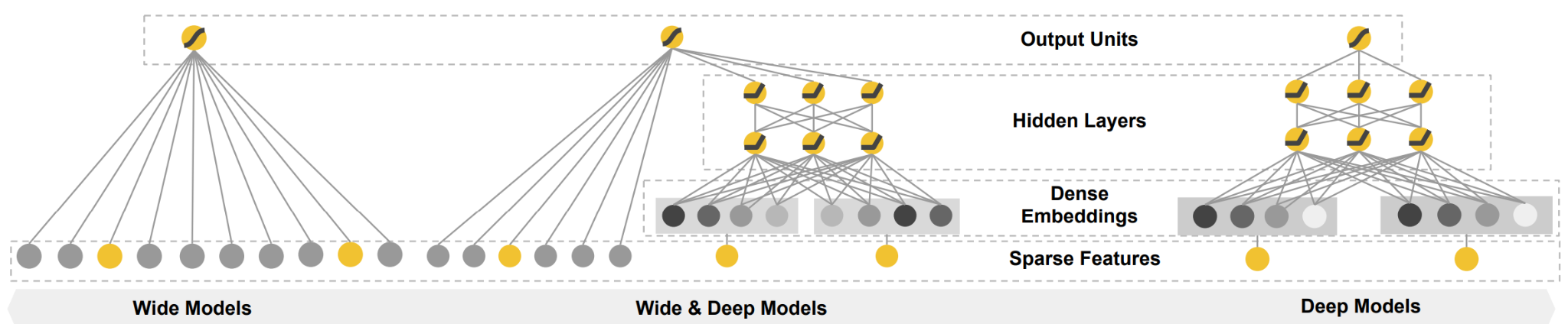
• Deep Crossing (Microsoft, 2016)^[12] and Wide & Deep (Google, 2016)^[13]: Deep Crossing is one of the early explorations to use DNN for recommendation. It proposes a classic structure with three types of layers stacked on top of each other: embedding layer, MLP layer (often with residual connection), and output scoring layer. Around the same time, the landmark Wide & Deep paper from Google introduced a framework that became a de factto template for many subsequent models. As illustrated in Figure 3, it explicitly combined two components: a "wide" part, which was a generalized linear model (like logistic regression) trained on raw features and their cross-products, and a "deep" part, which was a standard feed-forward neural network (DNN) that learned low-dimensional embeddings for features and also follows the stacked embedding→MLP→scoring layers pattern in Deep Crossing. The wide component was responsible for memorization—learning the predictive power of simple, frequently co-occurring feature interactions. The deep component was responsible for generalization—exploring new, previously unseen feature combinations via its dense embeddings. By jointly training these two parts, the model could be both accurate and responsive to novel scenarios.

• Successors to Wide & Deep: The core idea of combining wide and deep components was highly influential, leading to a family of models aimed at enrich the "wide" part to perform automated feature processing.

  • Deep & Cross Network (DCN, 2017)^[14]. This model replaced the wide component with a "cross network" designed to explicitly and automatically learn high-order feature interactions. While effective, the cross network's complexity made it more difficult to implement and computationally expensive. Figure summarizes many improvements to DCN and representative ones are: DCNv2^[15] (with explicit cross connection), GDCN^[16] (with gated cross network), DCNv3 or FCN^[17] (fuse linear cross network and exponential cross network), and XCrossNet^[18] (explicit crossing model that learns dense-dense and sparse-sparse interactions separately. Not exactly branded as a DCN variant, but highly related).

  

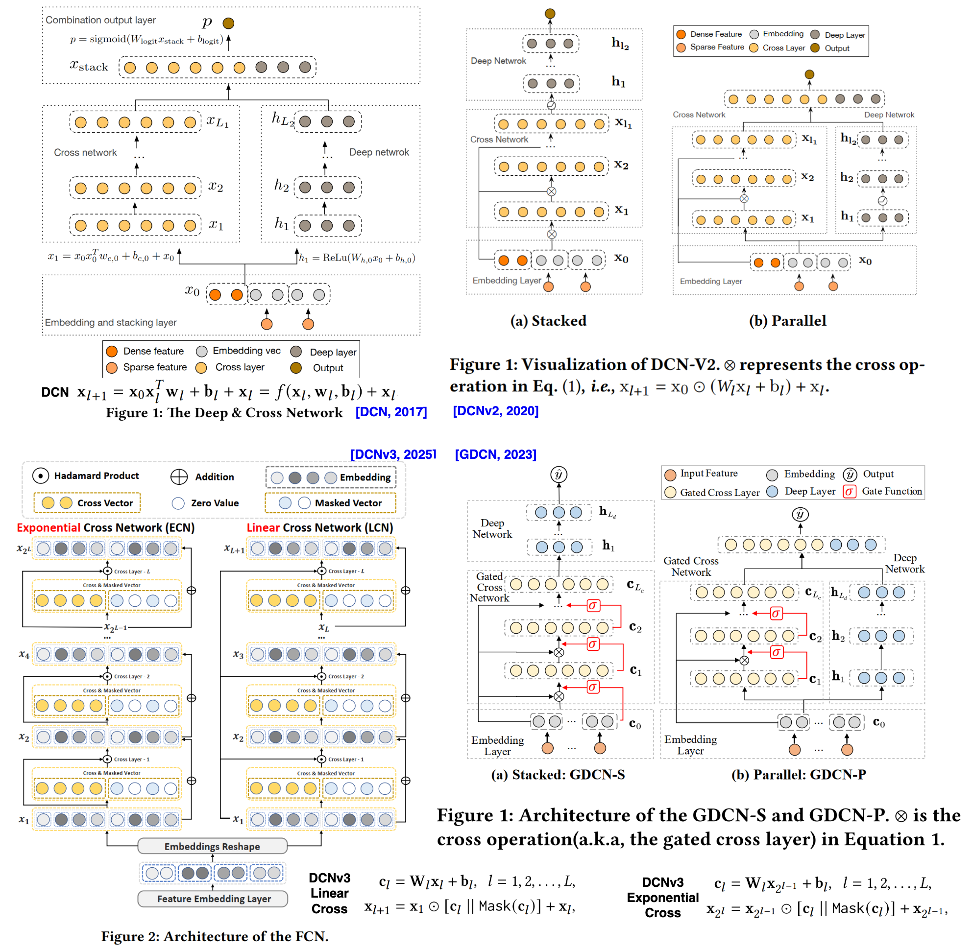
  The DCN(2017) established the modern hybrid learning-to-rank paradigm by explicitly introducing the Cross Network to efficiently model bounded high-order feature interactions, offering better performance than FMs and reduced feature engineering compared to Wide&Deep. Its limitations lay in the restricted expressiveness of the initial Cross Network when dealing with web-scale data, often deferring complex modeling to the parallel Deep Network. DCNv2 (2020) addressed these practical challenges by improving the expressiveness of the cross layer, enhancing the stability of the hybrid architecture, and incorporating practical deployment lessons learned from web-scale production systems. The subsequent GDCN(2023) prioritized interpretability, deeper crossing, and efficiency by introducing a Gated Cross Network (GCN) to dynamically filter noisy feature interactions and employing Field-level Dimension Optimization (FDO) to reduce redundant parameters in the embedding layer. The latest iteration, the Fusing Exponential and Linear Cross Network (FCN, 2025), also referred to as DCNv3, pushes the boundaries of explicit crossing by introducing the Exponential Cross Network (ECN) and Linear Cross Network (LCN) to achieve genuine, interpretable deep crossing, utilizing a self-mask operation to filter noise and demonstrating state-of-the-art results even without the implicit DNN component.

  • DeepFM (Huawei, 2017)^[19] This model offered a more elegant solution by replacing the manually engineered "wide" component with a Factorization Machine. The FM component and the DNN component share the same input feature embeddings. This design allowed DeepFM to learn both low-order (2nd-order) feature interactions via the FM part and high-order interactions via the deep part, without any need for manual feature engineering, simplifying the modeling pipeline.

• Two-Tower Architecture (from NeuralCF^[8] to widely adopted two-tower model architecture^[20]): Around 2017, the concept of Neural Collaborative Filtering (NCF) emerged, directly addressing a fundamental limitation of traditional Matrix Factorization (MF) methods: their reliance on a simple inner product to model user-item interactions. NCF innovatively replaced this fixed inner product with a neural architecture, specifically a MLP for the Neural CP layers in Figure 5, capable of learning arbitrary, complex nonlinear functions from data. This allowed NCF to capture more intricate and nonlinear relationships, leading to significant improvements in collaborative filtering performance. NCF also demonstrated its generality by showing that traditional MF could be interpreted as a special case within its framework.

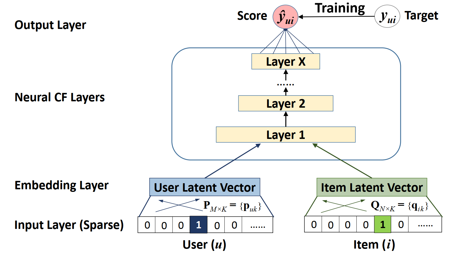
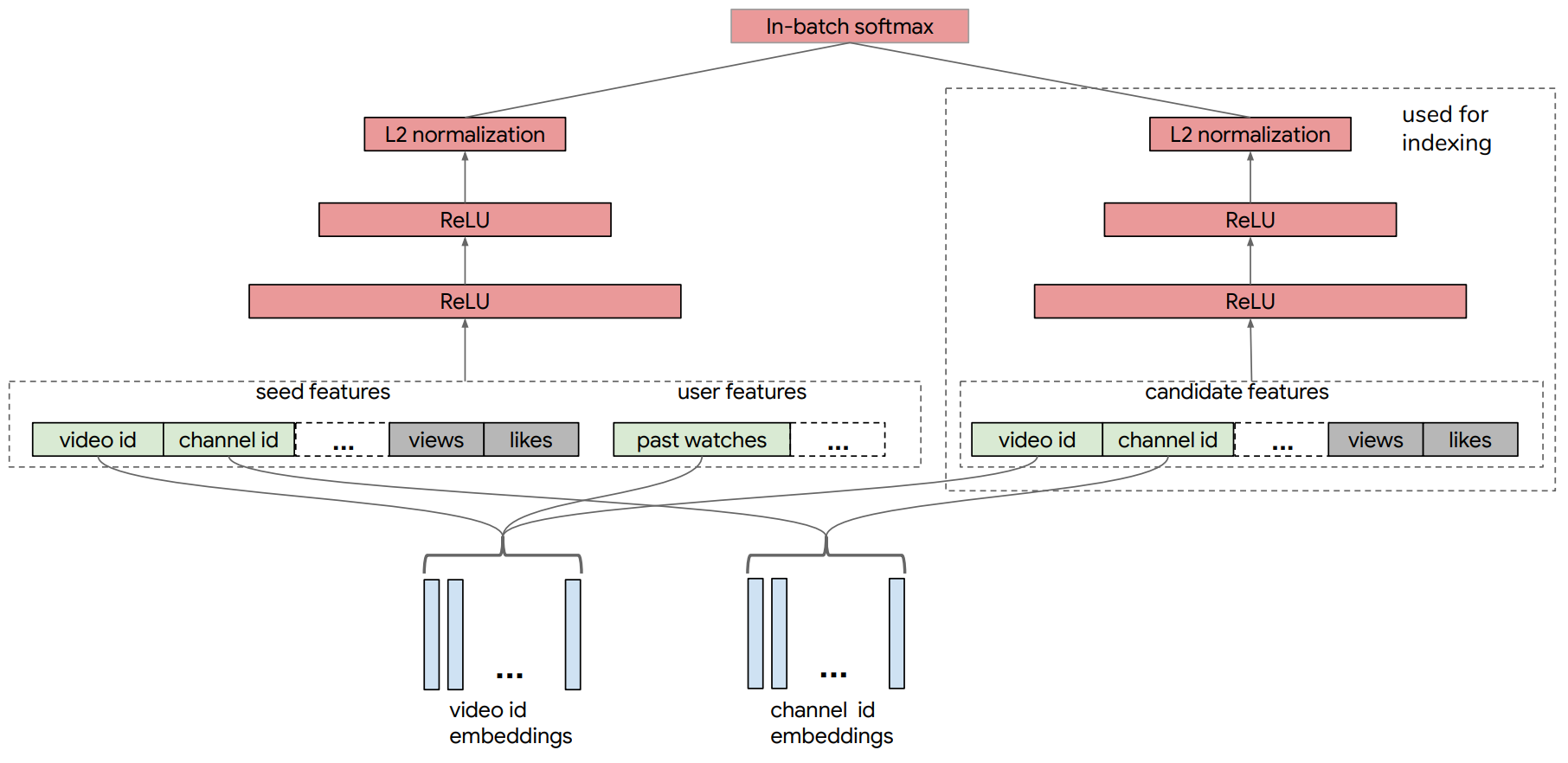
The evolution from NCF's approach to learning nonlinear interactions to the highly scalable Two-Tower Models (2TM) architecture represents a pivotal moment in solving the challenge of retrieving candidates from massive item catalogs. While NCF focused on applying deep layers to the combined user and item embeddings to learn a prediction score​, the subsequent two-tower model was driven by the industrial need for decoupled serving at scale and leverage more user and item features in addition to IDs. The 2TM, sometimes called a dual encoder, consists of two deep neural networks as shown in Figure 6: a User Tower and an Item Tower. Each tower independently processes its respective heterogeneous features to produce a single, dense embedding vector. The interaction function is then simplified to a computationally inexpensive dot product of these final embeddings. This architectural design enables the embeddings from the Item Tower to be precomputed and stored in a fast Approximate Nearest Neighbor (ANN) index, drastically reducing the real-time inference latency. This technique became the standard for the candidate retrieval stage, exemplified by the deployment of the retrieval system for large-corpus item recommendations (e.g., millions of videos on YouTube^[20]). The system further improved training stability and generalization by incorporating techniques like sampling-bias correction to account for the non-uniform distribution of item interactions in the training data.

• Neural Extensions of Factorization Machines: Another line of research focused on integrating neural networks directly with the FM architecture.
  • Neural Factorization Machines (NFM, 2017)^[21]: This model enhances the FM by adding a "Bi-Interaction" pooling layer after the embedding layer (Figure 7), which feeds the results of pairwise feature interactions into an MLP to capture nonlinear relationships.

• Attentional Factorization Machines (AFM, 2017)^[22]: AFM improves upon NFM by introducing an attention mechanism to the Bi-Interaction layer as shown in Figure 8. This allows the model to learn which feature interactions are more important for a given prediction, assigning higher weights to more impactful pairs.

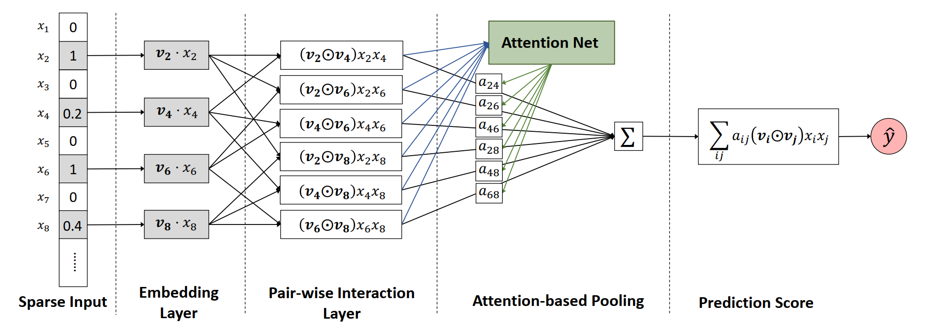
This is one of the earliest attempts to introduce attention into models for recommendation. The Attention Net in the diagram is a MLP with softmax output, and can be mathematically expressed in Equation (6).

where $\odot$ stands for element-wise product between two vectors, and the important model parameters for the two-layer MLP for Attention Net are $\mathbf{W} \in \mathbb{R}^{t \times k}$ for first layer model weights, $\mathbf{b} \in \mathbb{R}^{t}$ for first layer bias, and $\mathbf{h} \in \mathbb{R}^{t}$ for second layer model weights. The complete set of the pairwise interactions $a_{ij}'$ is then passed into softmax to get normalized attention weights $a_{ij}$. The attention weights determine which feature pair should have more weight for different input and the FM process in Equation (5) is upgraded to Equation (7).

Comparing to the standard attention mechanism in Equation (8)^[23],

AFM has the same matrix for $\mathbf{K}$ and $\mathbf{V}$, which is formed by cross operations of embedding vectors for the features, and the query matrix $\mathbf{Q}$ is the model weights W. It uses ReLU to shape the attention matrix instead of dividing by $\sqrt{d_k}$ in the original attention mechanism. But both have the same goal to stabilize the training process. Another interesting thing to note is that AFM does not introduce the candidate item or user behavior to shape the attention score. It mainly uses attention to improve inherent model capability. Intuitively, users actions on certain items are good indications about the relevance of the items and could be used to shape attention score calculation. This is the focus on many sequence modeling work that we will discuss in detail next.

Modeling User Dynamics and Attention: As model architectures matured, the focus shifted to a more challenging problem: modeling the dynamic, sequential nature of user behavior. A user's interests are not static; they evolve over time, and their actions form a sequence.

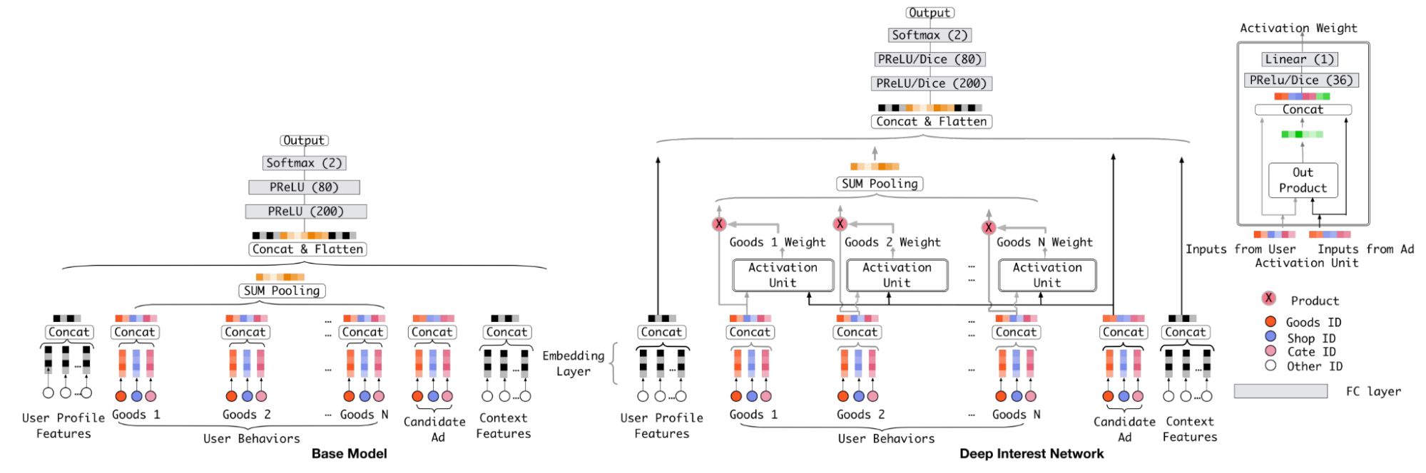
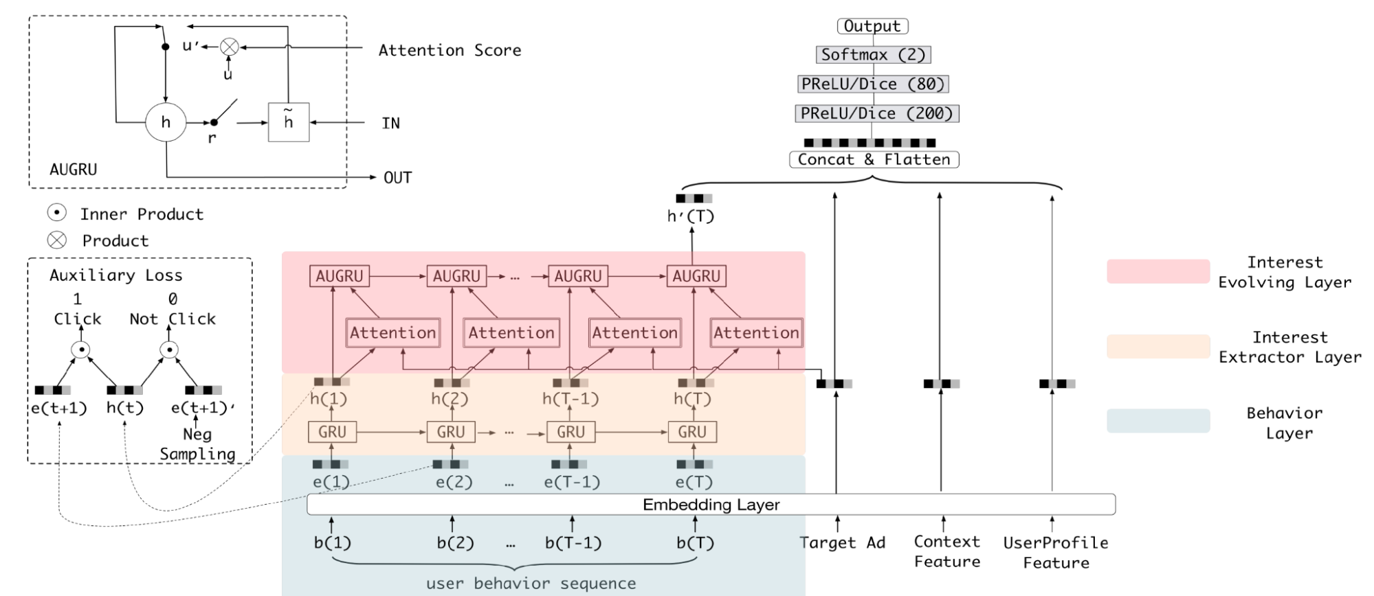
• Deep Interest Network (DIN, Alibaba, 2018)^[24]: This was a pivotal innovation, particularly for scenarios (social network, e-commerce, streaming, etc.) where user behavior histories can be long and diverse. The key insight behind DIN was that not all of a user's past behaviors are relevant to predicting their interest in a specific candidate item (Figure 9). For example, a user's interest in a new pair of running shoes is more influenced by their recent purchase of athletic apparel than their purchase of a kitchen appliance months ago. Previous models compressed the entire user history into a single, fixed-length vector, creating an information bottleneck. DIN introduced a local activation unit—effectively an attention mechanism—that adaptively calculates a user's interest representation. It computes the relevance between the candidate item and each item in the user's history, using these relevance scores to produce a weighted sum of the historical item embeddings. This creates a user representation that is dynamic and specific to the item being considered, significantly improving model expressiveness.

• Deep Interest Evolution Network (DIEN, Alibaba, 2018)^[25]: This model extended DIN by explicitly modeling the temporal evolution of user interests (Figure). It uses a sequential model (a GRU with an attentional update gate) to capture the dependencies within a user's behavior sequence, allowing it to better understand how interests change over time. However, this added complexity increased training time and online serving latency, thus requires strong engineering effort to host the model at scale.

• Self-Attention and Transformers: The groundbreaking success of the Transformer architecture in Natural Language Processing, based entirely on self-attention, quickly inspired its application to sequential recommendation.
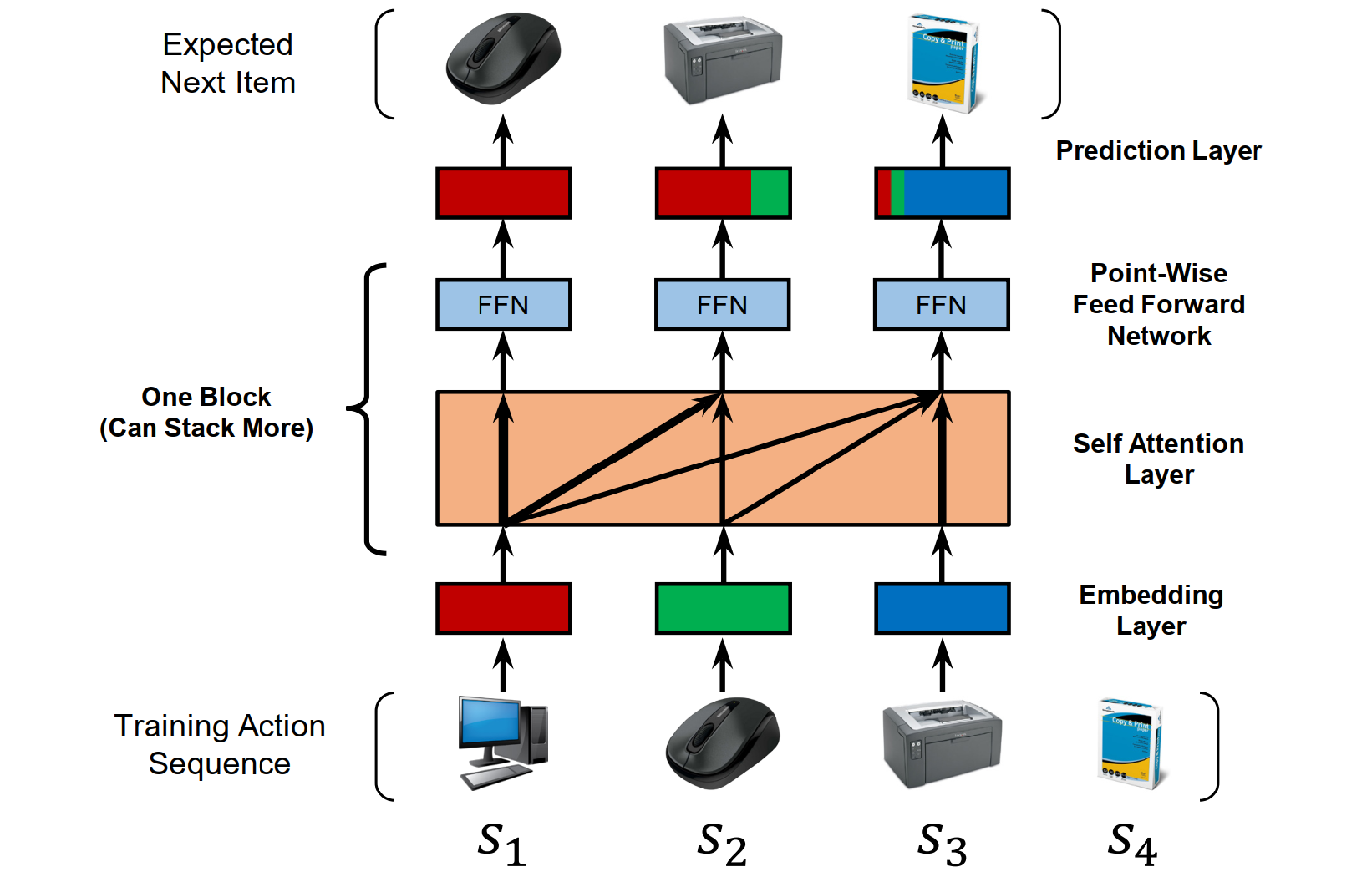
  • SASRec(2018)^[26]: The Self-Attentive Sequential Recommendation model was one of the first to successfully apply this idea (Figure 11). It treats a user's interaction history as a sequence of items, analogous to a sentence of words. The self-attention mechanism allows the model to weigh the importance of all previous items when predicting the next one. This enables it to capture complex, long-range dependencies within the sequence, outperforming prior methods based on Markov Chains, CNNs, or RNNs.

• BERT4Rec (2019)^[27]: Taking inspiration from the BERT model in NLP, BERT4Rec introduced a bidirectional self-attention model for recommendation (Figure 12). Traditional sequential models are auto-regressive, predicting the next item based only on past items (a left-to-right approach). BERT4Rec instead uses a "cloze" task, also known as a masked language model objective. During training, it randomly masks some items in the user's history sequence and then tries to predict those masked items, using both their left and right context (i.e., items that came before and after). This allows the model to learn deeper, richer contextual representations for items within a user's behavioral sequence. As a result, BERT4Rec has been widely used when causal relationships are not needed in the sequence.

  

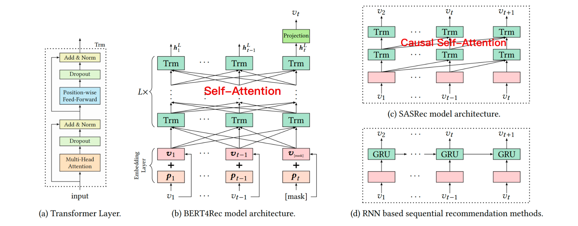
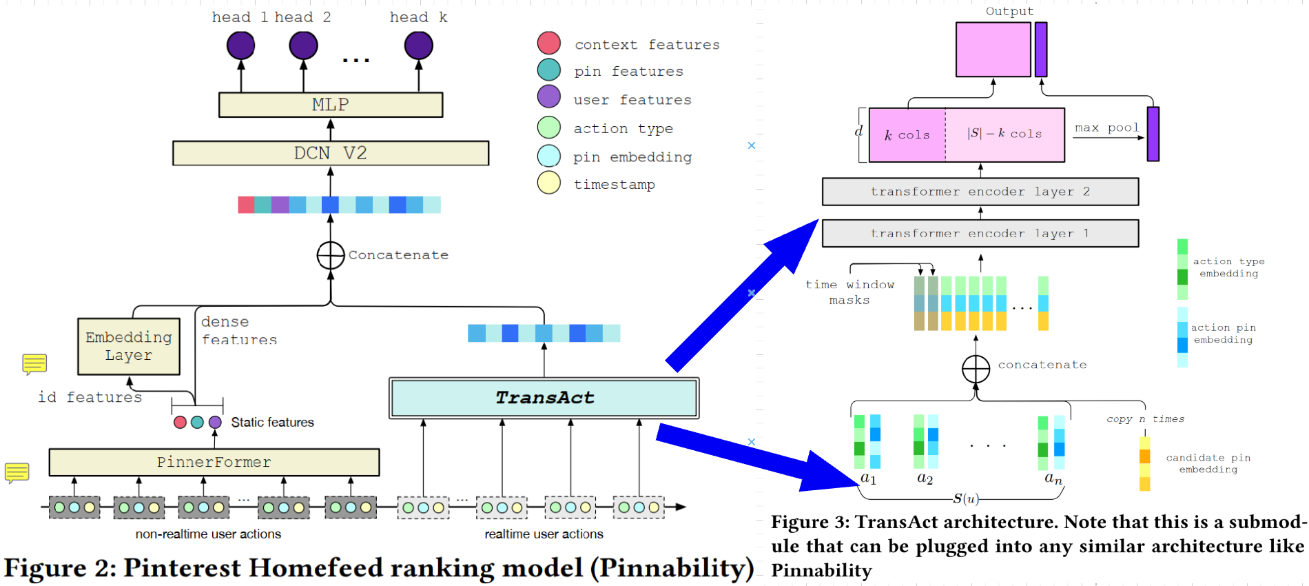
  • TransAct (Pinterest, 2023)^[28]: Representing a mature industrial application of these concepts, TransAct is a Transformer-based model designed for Pinterest's real-time ranking system (Figure 13). It employs a hybrid approach, combining short-term user preferences extracted from real-time activities with long-term interests learned from batch-generated user representations. A key innovation is its use of "early fusion," where the candidate item's embedding is concatenated with each item in the user's action history, allowing the model to explicitly learn the interactions between the candidate and the user's past engagements. This approach, while computationally intensive, delivered significant online engagement lifts but also introduced operational challenges, such as the need for frequent retraining to prevent model staleness and the initial drop in recommendation diversity, which was mitigated with a random time window mask during training.

Reinforcement Learning for Long-Term Value Optimization: Another significant paradigm shift within the deep learning era was the application of Reinforcement Learning (RL). This moved beyond optimizing for myopic, immediate rewards (like click-through rate) to maximizing long-term user value (LTV), such as sustained engagement, session length, or user retention. This is accomplished by framing the recommendation process as a sequential decision-making problem^[29], formally modeled as a Markov Decision Process (MDP), where the recommender system is an "agent" learning an optimal "policy" by interacting with the user "environment", and the reward either comes from user feedback or reward model.

• Balancing Exploration and Exploitation: A core challenge in dynamic systems is the trade-off between exploiting known user preferences and exploring new items to discover latent interests and avoid filter bubbles or echo chambers that trapes users in a narrow view of content by only recommending things they already like^[29]. Early approaches used contextual multi-armed bandits, which adapt to user feedback in real-time. For example, Yahoo! famously used a bandit approach for its news recommendations^[30], while Netflix applied it to personalize artwork and movie thumbnails, continuously learning the best presentation for each user to reduce regret from slower batch-based A/B testing^[29]. While effective, bandits are primarily suited for stateless problems and are limited in their ability to plan for the long-term consequences of actions. Full RL, which models state transitions and future rewards, addresses this but introduces new complexities, particularly the risk of deploying unstable policies in live production environments.
• Reinformance learning in real-world systems: A major hurdle for applying RL in modern recommenders is the slate-based interface, where a list of items is presented simultaneously. This creates a combinatorial action space; for a catalog of thousands of items, the number of possible slates is astronomically large, making standard RL methods intractable.

  • SlateQ (Google, IJCAI 2019)^[31]: The SlateQ framework, developed at Google for YouTube recommendations, was a breakthrough that made value-based RL practical for industrial systems. Its core innovation was to decompose the value of a slate into a tractable function of the values of its individual items. Under some practical assumptions about user choice—for instance, that a user selects at most one item from a slate—the Q-value of a slate could be expressed as the expected Q-value of its constituent items, weighted by their choice probabilities. This transformed the intractable problem of learning values for billions of slates into the manageable problem of learning values for individual items, enabling the use of temporal-difference learning algorithms like Q-learning at scale.

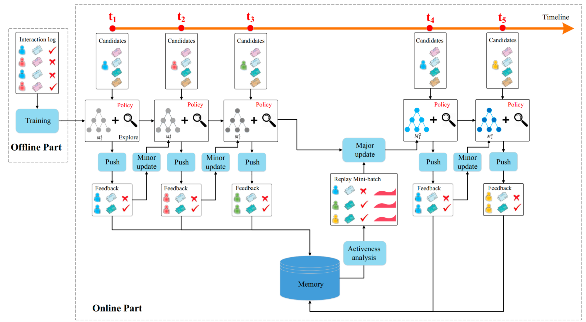
  • DRN (Microsoft, 2018)^[32]: The Deep Reinforcement Learning Framework for News Recommendation (DRN, 2018) was a seminal work that applied Deep Q-Learning to the sequential recommendation problem. DRN reframed the recommendation system as a sequential decision-making process: the system is the Agent, the user's browsing history and feature attributes constitute the State, and the decision to display a news item is the Action. The Reward incorporates both the immediate reward (click/no click) and a future reward, explicitly modeling the long-term impact on user behavior, such as a user's return pattern (how frequently the user comes back to the platform). This framework addresses the critical problem of maximizing future rewards and incorporating more subtle user feedback than just click labels. Furthermore, DRN incorporated an effective exploration strategy to avoid recommending only similar, popular news items, thereby mitigating user boredom and ensuring the discovery of new, attractive content.

    As illustrated in Figure 14, the DRN framework operates with two closely integrated components: offline pre-training and online continuous learning. Further, The alternating strategy of minor and major updates is a key insight of DRN, balancing adaptability with stability:

    • Minor Update: This strategy focuses on real-time adaptation to the immediate dynamic environment. It ensures the model's policy stays current with rapidly changing content and short-term user intent, preventing the policy from quickly becoming stale.
    • Major Update: This process focuses on stable, long-term learning. By sampling a diverse batch from the long-term memory, it breaks correlations in sequential observation data and performs deep, stable updates. This prevents catastrophic forgetting and ensures the model accurately learns the long-term return function, which is critical for maximizing user activeness and long-term utility. The overall structure effectively ensures that the model is constantly optimized both for the current context (minor updates) and for fundamental long-term user satisfaction (major updates).

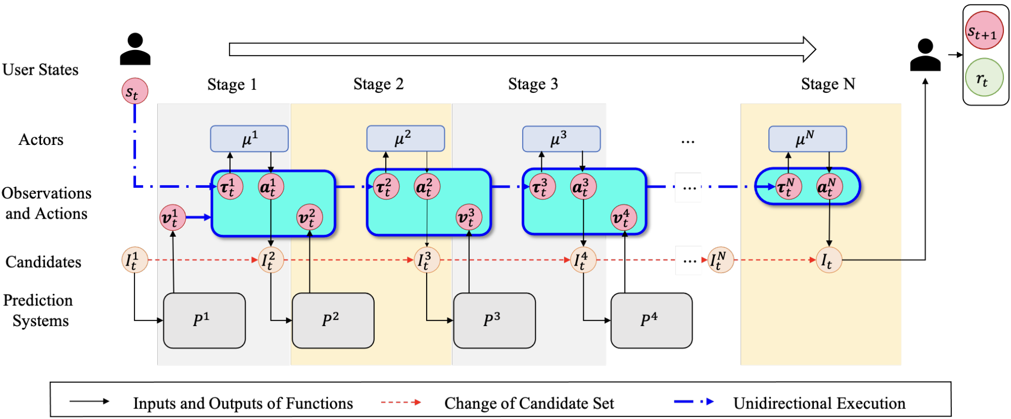
• UNEX-RL: Optimizing Multi-Stage Systems (Kuaishou, AAAI 2024)^[33]: Industrial recommenders are typically multi-stage pipelines (retrieval, ranking, re-ranking). The UNEX-RL framework is a multi-agent RL approach designed to jointly optimize all stages simultaneously (Figure 15). It treats each stage as a separate agent and addresses the unique challenges of this unidirectional architecture, namely "observation dependency" (an upstream action changes the input for all downstream stages) and the "cascading effect" (the policy gradient must account for an action's influence on all subsequent agents). Its reported online A/B test wins in a large-scale industrial system highlighting its real-world impact.

• The Challenge of Offline RL: A primary reason full RL deployments remain rare is the difficulty of offline training. Policies trained on static, historical logs often fail when deployed online due to a "distribution shift"—the new policy's actions generate data from a different distribution than the one it was trained on, leading to poor performance^{[@chen2024unex]}. This is a critical safety and stability concern. Current research is exploring ways to mitigate this, such as using conservative Q-learning, developing more robust off-policy evaluation methods, or even using Large Language Models (LLMs) as high-fidelity user simulators to generate more realistic feedback for offline policy training which we will touch more in the Generative Era.

Latent Representation Simplifies Feature Engineering #

For feature engineering, the Deep Learning Revolution directly addresses the limitations of manual feature engineering. It represented the first major step in offloading the work of feature discovery from humans to the model itself, a clear move towards leveraging computation.

In addition to continued automation of feature engineering and feature extraction with models, another core innovation was the embedding techniques. Instead of engineers manually creating sparse feature crosses, deep neural networks could automatically learn dense, low-dimensional vector representations (embeddings) for high-cardinality categorical features like user and item IDs. Word2vec laid the foundation work for embeddings including the embedding model architecture, training objective, and negative sampling techniques^[34],^[35].

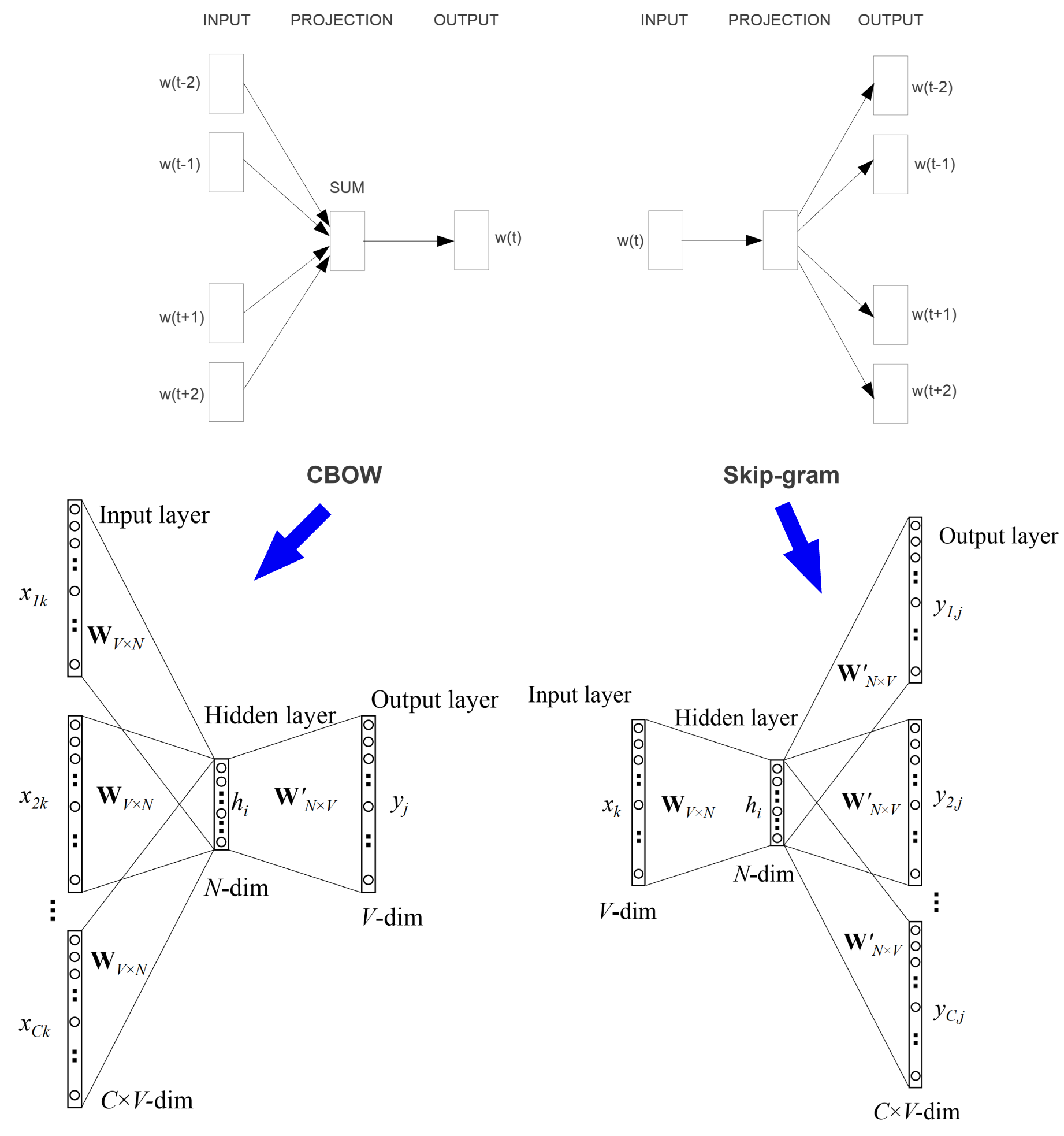
Figure 16 depicts two model architectures for word2vec embedding generation: continuous bag-of-word (CBOW) and skip-gram. In practice, the skip-gram generates better word embeddings and is used more often. One likely cause is that CBOW architecture directly sums or averages the word representations inside the network, and only the average is used for the word representation at the output to calculate loss. While in the skip-gram case, each word representation is directly used to calculate the loss. Although both models generate the aggregated word representations, the indirect aggregation via weight update through backpropagation in skip-gram results in higher-quality embeddings.

In both architectures, the W matrix contains embedding vectors at input space, with each row representing one word; the W' matrix contains embedding vectors at output space, with each column representing one word. The standard practice is to use W as the final embedding vectors. There are cases that achieve better performance for specific tasks by using some variants such as average $(W + W'^T)/2$ or even concatenation $[v_w; v'_w]$, but results are not consistent across tasks.

These foundation embedding techniques have been used to generate various embedding for items, users, and other related concepts in recommender systems such as search queries, carousel placements. Item2vec and node2vec are two representative use cases.

item2vec^[36]: item2vec extends word2vec from words to a list of items a user has engaged before. Assuming an item engagement list of length K in user history record $[w_1, w_2, w_3, …, w_K]$, similar to word2vec, the objective function item2vec is:

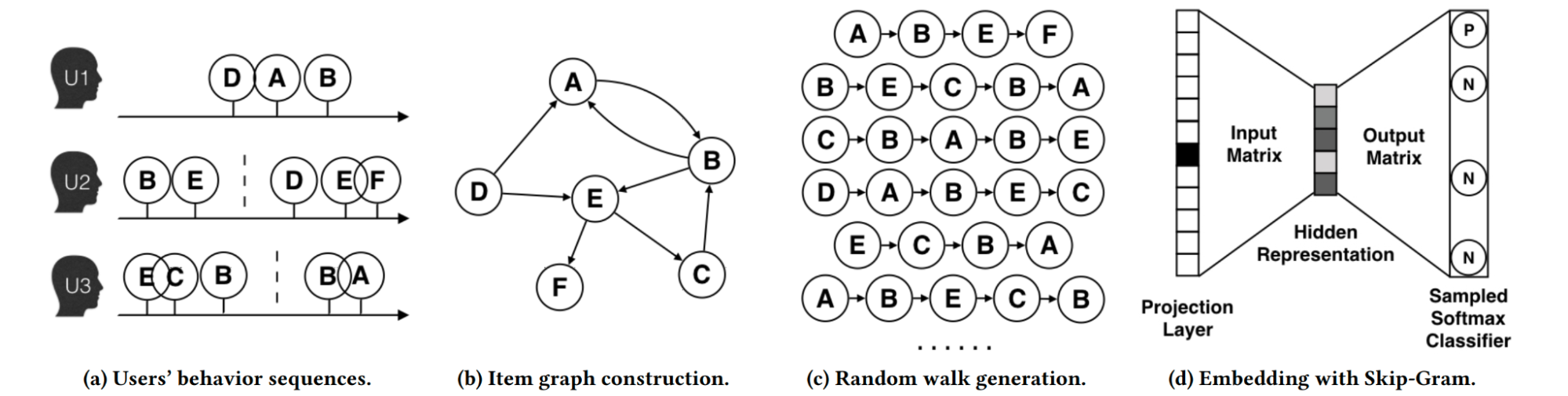
The only difference is that item2vec has removed the context window or time window. It assumes any two items are relevant to each other. Therefore, the objective function is the sum of log-loss for all pairs, not only pairs within a certain window. The training process for item2vec is exactly the same as word2vec. And the final item embedding lookup table is the same as the word representation W as illustrated in Figure 16. Item2vec has greatly expanded the application scenarios for word2vec, but its limitation is that only sequence item IDs are used to create embeddings. The connections among items and through user engagements are not captured. This overall relationship closely resembles a graph and node2vec that is developed to generate embedding for the relation graph.

node2vec^[37]: node2vec is an extension of a graph embedding technique named DeepWalk^[38], which is a direct improvement for item2vec to capture information beyond a user sequence. As illustrated in the Figure 17, the step c and d in DeepWalk is basically item2vec. The difference is that DeepWalk constructs an item graph through user behavior sequence in step a and b.

Node2vec further improves DeepWalk by adding more controls on random walk. As a result, the generated graph embedding can achieve a better balance between two kinds of similarities that are important for predictive tasks on nodes in networks: homophily and structural equivalence.

Specifically, under the homophily hypothesis, nodes that are highly interconnected and belong to similar network clusters or communities should be embedded closely together (e.g.,nodes S1 and u in Figure 18 belong to the same network community). In contrast, under the structural equivalence hypothesis, nodes that have similar structural roles in networks should be embedded closely together (e.g., nodes u and S6 in Figure 18 act as hubs of their corresponding communities). Importantly, unlike homophily, structural equivalence does not emphasize connectivity; nodes could be far apart in the network and still have the same structural role. In real-world, these equivalence notions are not exclusive; networks commonly exhibit both behaviors where some nodes exhibit homophily while others reflect structural equivalence.

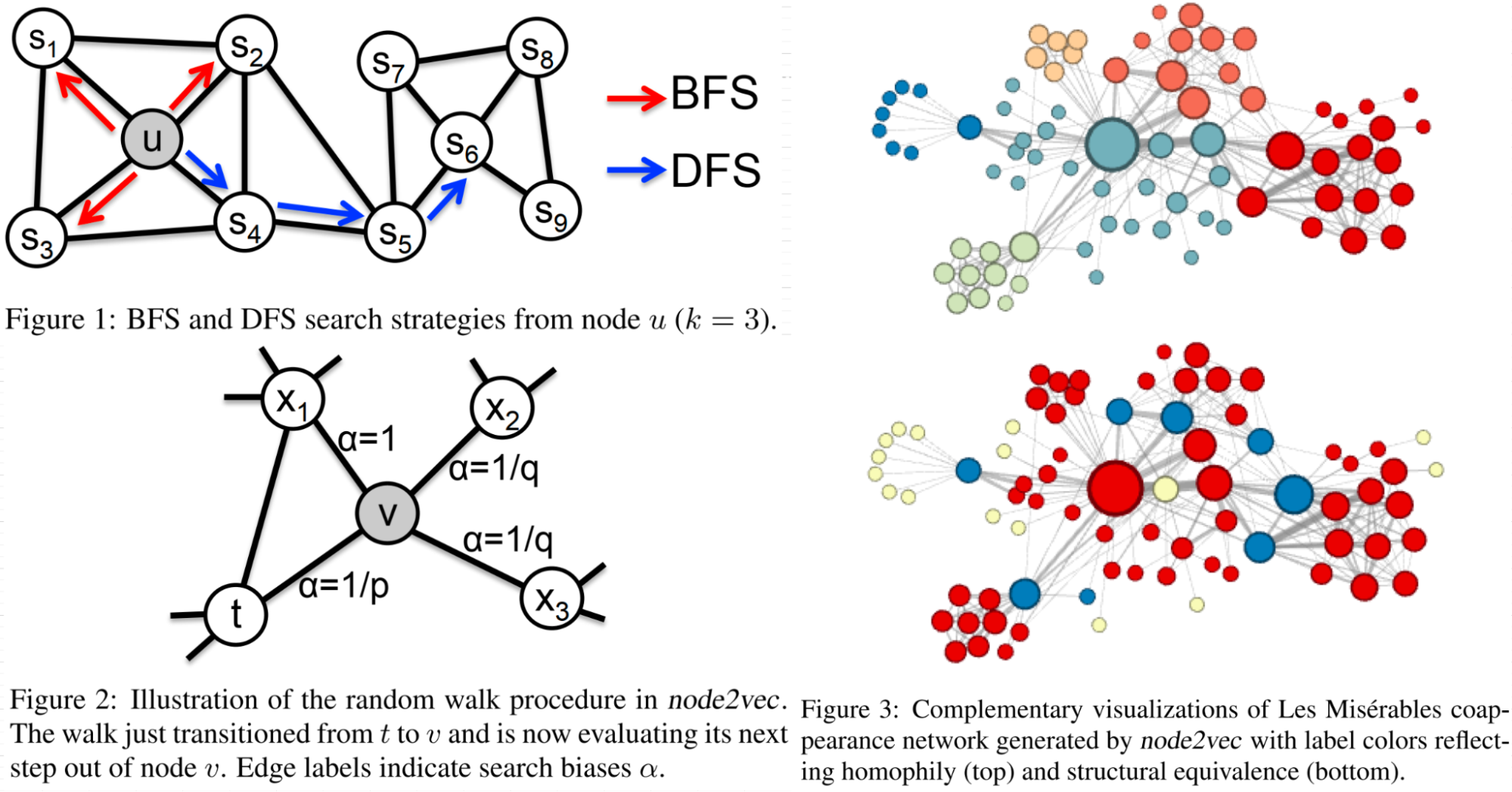
The work observes that BFS and DFS strategies play a key role in producing representations that reflect either of the above equivalences. In particular, the neighborhoods sampled by BFS lead to embeddings that correspond closely to structural equivalence. In order to ascertain structural equivalence, it is often sufficient to characterize the local neighborhoods accurately.

The opposite is true for DFS which can explore larger parts of the network as it can move further away from the source node u (with sample size k being fixed). In DFS, the sampled nodes more accurately reflect a macro-view of the neighborhood which is essential in inferring communities based on homophily.

With the above background in mind, how can we design a flexible neighborhood sampling strategy to allow us to smoothly interpolate between BFS and DFS? The node2vec work achieves this by developing a biased random walk procedure that can explore neighborhoods in BFS as well as DFS fashion. The biased random walk procedure is controlled by the transition probability as depicted in Figure 14, and the transition probability is defined in Equation (10):

where p and q are parameters for a second-order random walk, and $d_{tx}$ represents the shortest path distance between node t and x.

As a result, the generated embedding can be controlled by p and q; thus controlling the interpolation of BFS and DFS traversal process to express homophily and structural equivalence in the graph. Figure 15 contains two examples when the traversal process is set close to two ends of the spectrum.

Figure 18 (top right) shows the example with p = 1 and q = 0.5. Notice how regions of the network (i.e., network communities) are colored using the same color. In this setting node2vec discovers clusters/communities of characters that frequently interact with each other in the major sub-plots of the novel. Since the edges between characters are based on coappearances, we can conclude this characterization closely relates with homophily.

In order to discover which nodes have the same structural roles we use the same network but with p = 1 and q = 2, use node2vec to get node features and then cluster the nodes based on the obtained features. Here node2vec obtains a complementary assignment of nodes to clusters such that the colors correspond to structural equivalence as illustrated in Figure 18 (bottom right). For instance, node2vec embeds blue-colored nodes close together. These nodes represent characters that act as bridges between different sub-plots of the novel. Similarly, the yellow nodes mostly represent characters that are at the periphery and have limited interactions. One could assign alternate semantic interpretations to these clusters of nodes, but the key takeaway is that node2vec is not tied to a particular notion of equivalence. As shown through more experiments in the paper, these equivalence notions are commonly exhibited in most real-world networks and have a significant impact on the performance of the learned representations for prediction tasks.

As demonstrated in word2vec, item2vec, and node2vec above and many more examples in the embedding layers in model architectures discussed above, the embedding techniques can generate powerful and useful representations to help us build better recommender systems. This had several profound effects:

• Automated Feature Representation: The model learned the "features" of users and items as part of the training process, and stored in embedding vectors, capturing latent semantic relationships without human intervention. These embeddings are then used to retrieve items (known as embedding-based retrieval), or directly used as features to the deep learning models for ranking.
• Automated Feature Interaction: Architectures like DeepFM went a step further by combining the embedding concept with a Factorization Machine component, allowing the model to automatically learn both low- and high-order interactions between all input features, effectively replacing the manual cross-product transformations of the previous era.
• End-to-End Sequential Modeling: The rise of sequential models like SASRec and BERT4Rec meant that raw sequences of user behavior (e.g., a list of clicked item IDs) could be fed directly into the model. The Transformer architecture itself was responsible for learning the complex temporal patterns and feature interactions within the sequence, a task that was previously impossible without heavy preprocessing and feature creation.
• The Rise of AutoML: This trend towards automation culminated in the application of Automated Machine Learning (AutoML) techniques to recommender systems. Researchers began developing methods to automatically search for optimal embedding dimensions, select the most useful features, and even discover the best feature interaction architectures, further reducing the need for human expertise.

The Generative Era: Unifying Systems Through Scalable Learning #

The third and ongoing phase marks another significant paradigm shift in the history of recommender systems. The journey through the Classical and Deep Learning eras was a clear progression of the "Bitter Lesson": computation-heavy, general-purpose methods consistently overtook those reliant on human-curated knowledge and feature engineering. However, even the most advanced deep learning models in the DL era were fundamentally constrained. They excelled at learning from structured interaction data (user IDs, item IDs, clicks) but struggled to deeply understand the rich, unstructured world of content and the nuances of human intent. This created a ceiling on their ability to handle many problems such as cold-start, transparent explanations, and interactive dialogue.

The breakthrough came from an adjacent field: the rise of Foundation Models (FMs), particularly Large Language Models (LLMs), pre-trained on the vast content of the web. (Note: In this section, "FM" refers to Foundation Models, not to be confused with Factorization Machines from the earlier eras.) These models demonstrated an unprecedented ability to understand semantics, reason, and generate human-like language. Their emergence provided a path to shatter the previous ceiling, ushering in the Generative Age. This era represents a deeper expression of the Bitter Lesson, defined by a move away from specialized models for different tasks toward the vision of a single, massive, general-purpose learning machine that learns directly from the richest and most diverse data possible.

The Paradigm Shift: Enablements for the Generative Era #

The adoption of Foundation Models in recommender systems is not merely an incremental improvement but a fundamental rethinking of what a recommender can be. This shift is driven by a set of new capabilities that were previously out of reach for traditional models^[3].

1. Enhanced Generalization: Conquering Cold-Starts and Data Sparsity
   Traditional models learn about items primarily through user interactions, leaving them blind to new or niche content (the "cold-start" problem). Foundation Models possess deep semantic knowledge. They can understand an item based on its description, image, or attributes alone, without any interaction data. This allows them to infer relationships and make relevant recommendations for brand-new items, effectively solving the cold-start issue. This is a direct manifestation of the Bitter Lesson: achieving robust generalization not through clever algorithms for sparsity, but through the scalable learning of a massive, general-purpose model that has ingested a significant portion of human knowledge.
2. Transformative User Experience: From Static Lists to Dynamic Conversations
   For decades, the recommendation experience has been a one-way street: a system presents a static list, and the user consumes it. FMs, with their mastery of natural language, enable a transformative shift toward dynamic, interactive, and conversational experiences. Instead of passively receiving recommendations, users can engage in multi-turn dialogues, ask clarifying questions ("Can you find me something like this, but less serious?"), and provide nuanced feedback in their own words. This moves beyond the rigid constraints of clicks and ratings, allowing for a more natural and collaborative user journey where the system can adapt in real-time to a user's evolving intent.
3. Transparent Reasoning: Unlocking the 'Why' Behind Recommendations
   A long-standing challenge for recommender systems has been their "black box" nature. Explanations were often simplistic and template-based (e.g., "Users who liked X also liked Y"). Foundation Models, with their emergent reasoning abilities, can generate coherent, context-rich, and personalized explanations for their suggestions. By leveraging their world knowledge, they can connect a user's preferences to an item's attributes in a deeply semantic way (e.g., "Because you enjoy historical fiction with strong female protagonists, you might like this book"). This ability to articulate the "why" behind a recommendation fosters user trust and provides a more satisfying and interpretable experience.

Underpinning this entire shift is a fundamental change in how systems handle data. Traditional recommenders primarily operate on structured data: user and item IDs, demographic attributes, and explicit or implicit feedback logs. Foundation Models excel at processing diverse, multimodal data, unifying text, images, audio, and even network graph data into a cohesive understanding. This allows the system to learn from a much richer and more holistic representation of the world, letting massive computation find the latent structure in the most general data available—the core tenet of the Bitter Lesson.

Three Emerging Paradigms of Foundation Model-Powered RecSys #

The integration of Foundation Models into recommender systems is unfolding across a spectrum of approaches and the industry is collectively exploring different directions. These can be understood as three distinct but interconnected paradigms, each representing a progressively deeper commitment to leveraging large-scale, general-purpose computation over specialized, human-designed components.

Feature Paradigm #

In the most common and pragmatic approach today, FMs act as a powerful component within a traditional architecture. This paradigm focuses on using FMs to make existing Deep Learning Recommendation Models (DLRMs) better, either by improving their inputs or enhancing their architecture.

• FMs as Feature Engineers: In this role, FMs serve as universal feature extractors. They transform raw, unstructured data into high-quality, semantically rich features that are then fed into conventional DLRMs.
  • Semantic IDs (TIGER^[39] and YouTube Video^[40]): Google has introduced semantic IDs and tested them in both public real-world benchmarks (TIGER) and YouTube Video. Taking YouTube for example, to tackle the cold-start problem for new videos, YouTube uses a powerful transformer-based video encoder to generate a content embedding, which is then compressed into a sequence of discrete tokens called a "Semantic ID." This ID captures the video's semantic essence and is used as a feature in their product retrieval and ranking models, significantly improving performance for new videos before they accumulate interaction data.

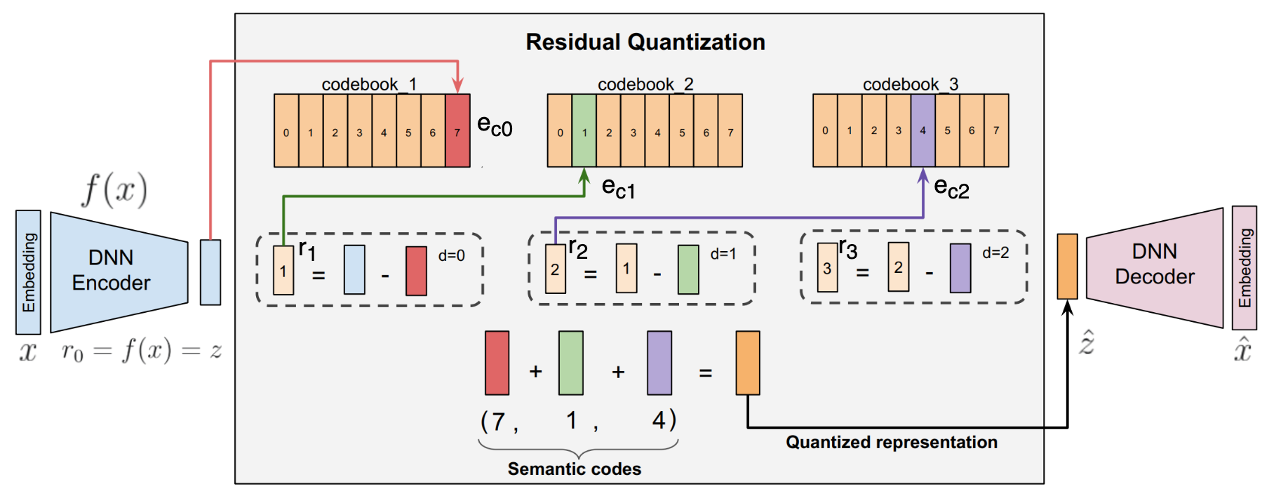
The semantic ID creation is an iterative process and Figure 19 summarizes the typical flow with the Residual Quantized-Variational AutoEncoder model. The RQ-VAE is a multi-level vector quantizer that applies quantization on residuals to generate the tuple of codewords (i.e. Semantic IDs). There are three jointly-trained components in semantic ID creation process:

1. an encoder $\mathcal\varepsilon$ that maps the input embedding $x \in R^{dx}$ to a latent vector $z \in R^{dz}$

2. a residual quantizer with $m$ levels to recursively quantize the residual to the nearest codebook vector

3. a decoder $\mathcal{D}$ that maps the quantized latent $\hat{z}$ back to the original embedding space $\hat{x}$.

Here is a brief summary about the semantic ID creation process. Given the embeddings (often created by some general-purpose embedding models like Sentence Transformer, BERT, etc.) as input $x$, the autoencoder converts that into a latent representation $z=\epsilon(x)$. It is also denoted as $r_0$, the initial residual at the zero-th level ($d=0$). At each level $d$, there is a codebook $C_d = \{{\mathbf{e}_k}\}_{k=1}^K$ where $K$ is the codebook size. At zero-th level, $r_0$ is quantized by mapping it to the nearest embedding from that level's code book. The index of the closest embedding $e_{c_0}$, i.e., $c_0 = \text{argmin}_i\|r_0 - e_k\|$, represents the zero-th level codeword. Similarly, the code for the first level is computed by finding the embedding in the codebook for the first level which is nearest to $\mathbf{r}_1$. The process is repeated recursively $m$ times to get a tuple of $m$ codewords that represent the Semantic ID.

Once we have the semantic ID ($c_0,.,c_{m-1}$), a quantized representation of $z$ is computed as $\hat{z} = \sum\nolimits_{d=0}^{m-1}e_{c_d}$ . The $\hat{z}$ is passed to the decoder, which tries to recreate the input $x$ with $\hat{z}$. The RQ-VAE loss is defined in Equation (11):

Here $\hat{x}$ is the output of the decoder, and $\text{sg}$ stands for stop-gradient operation. The loss jointly trains the encoder, decoder, and the codebook.

Let's get some insights for the overall loss function. The $\mathcal{L}_{\text{recon}}$ is the standard reconstruction loss of an autoencoder. The $\mathcal{L}_{\text{rqvae}}$ is the loss related to the residual quantization process and this is the interesting part. $\mathcal{L}_{\text{rqvae}}$ encourages the encoder and the codebook vectors to be trained such that $\mathbf{r_d}$ and $\mathbf{e_{c_d}}$ move towards each other, and stop-gradient help achieve this.

Specifically, one part is named codebook update term: $\|\mathbf{sg[r_d] - e_{c_d}}\|^2$. Gradient flows only to $\mathbf{e_{c_d}}$ in order to move it towards the current residuals, similar to the center update step in the k-means algorithm.

The other part is commitment term $\beta\|\mathbf{r_d} - sg[e_{c_d}]\|^2$. Gradient flows only to $\mathbf{r_d}$: the encoder is nudged to commit to the chosen code, not to move the code around.

Hypothetically, if there is no stop-gradient, the second part of the loss reduces to $\mathcal{L}_\text{rqvae} = \|r - e\|$, omitting the constant scaling factor $\beta$ and level $d$ for simplicity. The gradient backpropagation process during training could lead to mutual chasing issues between $\mathbf{r}$ and $\mathbf{e}$. Here is why mutual chasing happens.

With the reduced loss function, the gradients for $r$ and $e$ are

$\nabla_r \|r - e\|^2 = 2(r - e), \quad \nabla_e \|r - e\|^2 = -2(r - e)$

With learning rate $\eta_r > 0$ and $\eta_e > 0$, we have

The distance between $r$ and $e$ after gradient update is:

$\Delta_{t+1} =r_{t+1} - e_{t+1}= (1 - 2(\eta_r + \eta_e)) \Delta_t$

So the distance shrinks (great!), but the center drifts:$\frac{r_{t+1} + e_{t+1}}{2} = \frac{r_t + e_t}{2} + (\eta_e - \eta_r) \Delta_t$

Unless $\eta_r = \eta_e$ and nothing else acts on $r$, the pair ($r$,$e$) walks around: $e$"chases" $r$ (which is itself moving due to reconstruction gradients), rather than anchoring to the data distribution. On a mini-batch, each step pulls $e$ towards wherever the encoder currently emits $r$ (which can fluctuate batch-to-batch), making the codebook a moving target instead of a stable set of cluster centers.

In practice, the codes drift with encoder quirks or reconstruction gradients, assignments are noisy across steps, and some codes never get any stable mass (collapse risk), others become "sticky" by accident.

• LLM-Assisted Data Generation. FMs are also being used to generate high-quality data for other models. Bing uses GPT-4 to generate better titles and snippets for webpages to train its rankers, while Amazon and Spotify use LLMs to generate synthetic user queries to address data scarcity. Here, the FM acts as a scalable source of domain expertise, automating a critical part of the data pipeline. Yan's blog^[41] did a good summary on this topic, and please refer to that for more details.
• FMs as Architectural Components: FMs can also enhance the model architecture itself, often by aligning different types of representations.
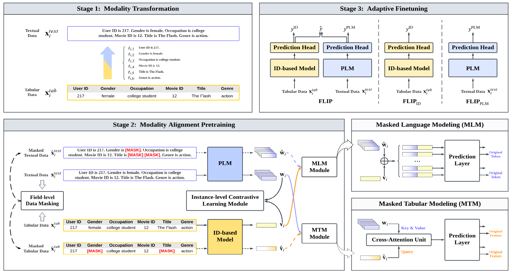
  • Case Study: Huawei's FLIP Framework^[42]: This framework aligns a traditional ID-based recommendation model with an LLM (Figure 20). It jointly trains the two models, forcing them to produce aligned embeddings by reconstructing masked features from one modality (e.g., user/item IDs) using information from the other (text tokens) ([41] also has a good summary with more details on this). This hybrid approach leverages the LLM's rich content understanding to improve the representations in the ID-based model.

Generative Paradigm #

The generative paradigm represents a more radical architectural shift. Here, the FM is not just a component but becomes the core recommendation engine itself. It moves beyond predicting scores and instead directly generates the recommended items, their explanations, or conversational responses. More importantly, the industry is also trying to answer a critical question: Does scaling law in language models apply to models for the recommender system? In other words, can we build foundation models for recommender systems to gain better performance by scaling up model parameters?

• The Generative Leap: The foundational change is the reformulation of the core algorithmic objective. Conceptually, the model moves from learning a discriminative function $\mathbf{P}\textbf{(click}|\textbf{user, item)}$ to learning a generative distribution $\mathbf{P}\textbf{(item}|\textbf{user, history)}$.
• Unifying the Pipeline: Vision vs. Reality: A central ambition of this paradigm is to replace the entire retrieval-ranking-reranking pipeline with a single, end-to-end generative model. However, the immense compute and latency constraints of real-time serving mean that the functional separation of retrieval and ranking often persists in practice. The current landscape is therefore one of a phased transformation, where generative components are replacing or augmenting their discriminative counterparts stage by stage. Let's dive into a few representative case studies.
• Case Study: Meta's HSTU for GR^[43]. Meta's work on Generative Recommendation (GR) has applied the generative paradigm into the production system for the critical retrieval and ranking tasks, with many interesting contributions in the feature engineering, HSTU model, and efficient model serving.
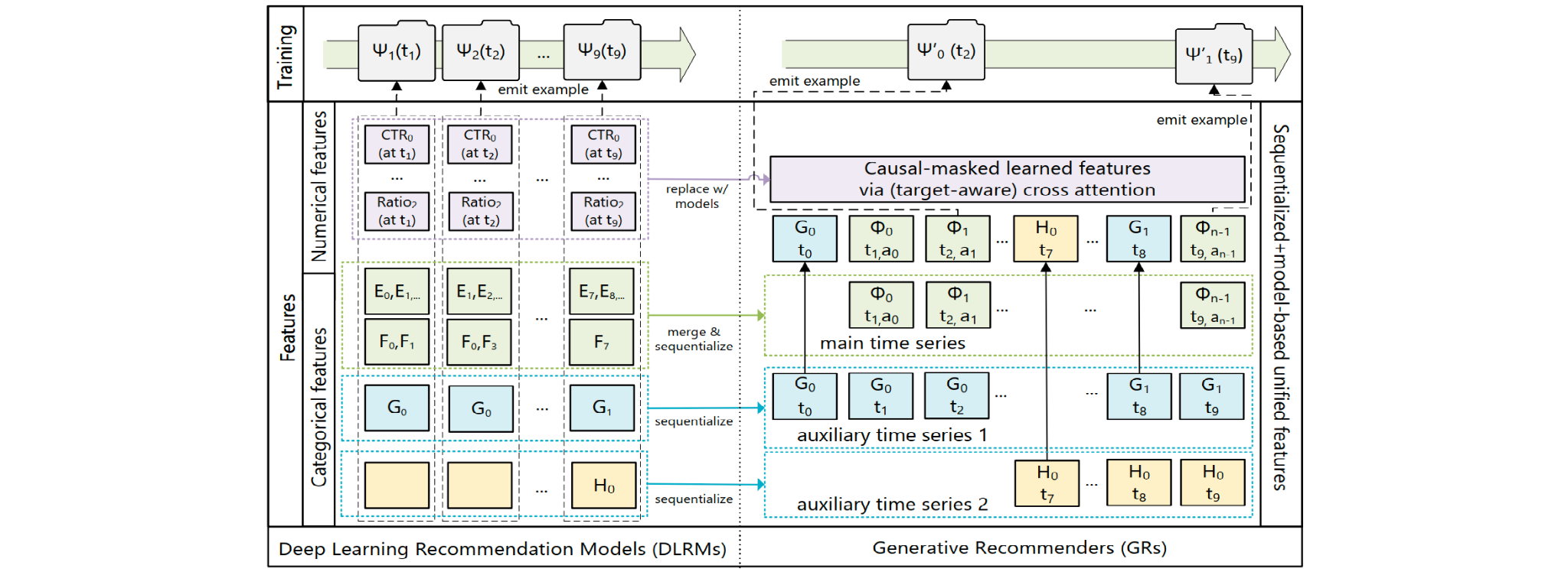
  1. User Sequence as a New Modality: Inspired by the scalability in LLM through vast amounts of internet data, this work brings explicit structure to organize features, aiming to achieve a similar effect for recommender systems. Specifically, the work treats user actions as a new modality and encodes these features into a single unified time series as depicted in Figure 21. This is a profound extension of feature engineering in the sequential recommendation that we discussed above. For the numerical features such as weighted/decayed counter, ratios, cross features, etc., since they can potentially change with every single user-item interaction, it is infeasible to fully sequence such features from computation and storage perspective. However, an insightful observation is that GR models can implicitly learn these numerical features through the sequentialization with target-aware formulation, aggregation and encoding of categorical features (e.g. item topics, locations, actions), given enough dataset samples and sufficiently expressive model. Therefore, numerical features could be removed in the sequence.

2. Recommendation Tasks Reformulation: The paper reframes standard retrieval and ranking tasks into the following generative tasks (noted as sequential transduction tasks) in Table 1. Given a list of $n$ tokens $x_0, x_1, \cdots, x_{n-1} \quad (x_i \in \mathbb{X})$ ordered chronologically and the time when those tokens are observed $t_0, t_1, \cdots, t_{n-1}$, the generative task maps this input sequence to the output token $y_0, y_1, \cdots, y_{n-1} \quad (y_i \in \mathbb{X} \cup \{\emptyset\})$ where $y_i = \emptyset$ indicates that $y_i$ is undefined. Further, $\Phi_i \in \mathbb{X}_c \quad (\mathbb{X}_c \subseteq \mathbb{X})$ denote a content item (e.g., images or videos) that the system provides to users. Since new contents are constantly created, $\mathbb{X}_c$ and $\mathbb{X}$ are non-stationary. Users can engage with $\Phi_i$ with some action $a_i$ (e.g. like, share, comment, skip) and $a_i \in \mathbb{X}$. The total number of contents a user has engaged with is denoted by $n_c$.

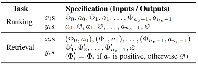
Table 1: Ranking and retrieval as sequential transduction tasks.Other categorical features are omitted for simplicity.

Retrieval: In retrieval stage, we learn a distribution $p(\Phi_{i+1}|u_i)$ over $\Phi_{i+1} \in \mathbb{X}_c$, where $u_i$ is the user's representation at token $i$. A typical objective is to select $\text{argmax}_{\Phi \in \mathbb{X}_c} p(\Phi | u_i)$ to maximize some reward. This differs from a standard autoregressive setup in two ways. First, the supervision for $x_i, y_i$ is not necessarily $\Phi_{i+1}$ since users could respond negatively to $\Phi_{i+1}$. Second, $y_i$ is undefined when $x_{i+1}$ represents a non-engagement related categorical feature, such as demographics.

Ranking: Ranking tasks in GRs pose unique challenges since industrial recommender systems often require a "target-aware" formulation. In such case, "interactions" of target, $\Phi_{i+1}$, and historical features need to occur as early as possible, which is infeasible with a standard autoregressive setup where "interaction" happens late (e.g. via softmax after encoder output). This is addressed by interleaving items and actions as shown in Table 1, which enables the ranking tasks to be formulated as $p(a_{i+1}|\Phi_0, a_0, \Phi_1, a_1, \cdots, \Phi_{i+1})$.

3. HSTU Model: In the modeling front, after reformulating recommendation as a sequential transduction task, the highly optimized Hierarchical Sequential Transduction Unit (HSTU) architecture is developed as illustrated in Figure 22. The HSTU model architecture takes inspiration from transformer, with many customizations based on insights from recommender systems:
   - Pointwise aggregated attention, non-softmax: Traditional softmax attention tends to wash out strong signals in long sequences. HSTU replaces this with pointwise attention (using SiLU), which preserves intensity and sharp signal contrast to capture intensive user preference and suit better for the non-stationary vocabularies in streaming settings.
   - Relative attention bias: By incorporating both position and time into attention bias, HSTU models become more aware of recency and behavioral patterns—something we know is crucial for recommendation.

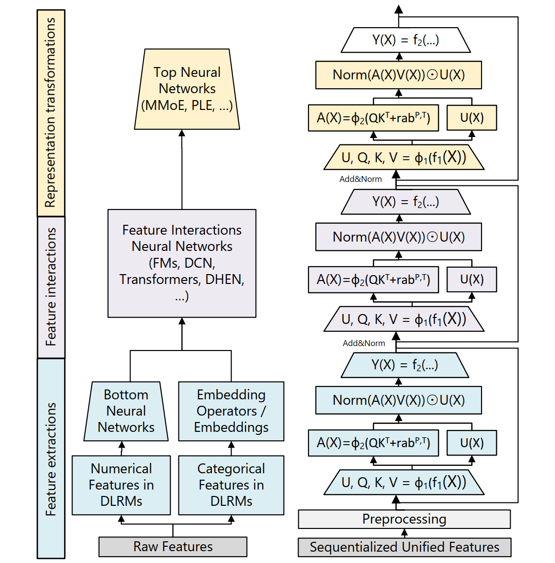
4. Efficient mode inference: There are many optimizations involved in the training and serving for the HSTU model. The same HSTU model is used for both retrieval and ranking. We highlight the optimization on model inference that enables Meta to rank thousands of items within time budget using the large HSTU model (claimed to have 1.5T parameters).

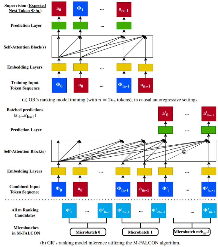
Note that the self-attention algorithm is modified such that $\Phi'_i$ cannot attend to $\Phi'_j$ when $i \neq j$ - this is highlighted with "X" in the figure.
Microbatched-Fast Attention Leveraging Cacheable OperatioNs (M-FALCON) is the key optimization algorithm as illustrated in Figure 23. In the forward pass, M-FALCON handles $b_m$ candidates in parallel by modifying attention masks and $b_m$ biases such that the attention operations performed for $b_m$ candidates are exactly the same. This reduces the cost of applying cross-attention from $O(b_mn^2d)$ to $O((n + b_m)^2d) =O(n^2d)$ when $b_m$ can be considered a small constant relative to $n$. We optionally divide the overall m candidates into $\lceil m/b_m \rfloor$ microbatches of size $b_m$ to leverage encoder-level KV caching45 either across forward passes to reduce cost, or across requests to minimize tail latency.
As a result, M-FALCON enables model complexity to linearly scale up with the number of candidates in traditional DLRMs’s ranking stages. The work succeeded in applying a 285x more complex target-aware cross attention model at 1.5x-3x throughput with the same inference budget for a typical ranking configuration in DLRM ranking system.

To summarize, the work demonstrated that a pure generative model could deliver 12% improvements in online A/B tests, significantly outperforming highly tuned DLRMs at massive scale for both retrieval and ranking tasks. It has also validated that, like the language models, the GR systems are much more scalable than DLRMs. This was the first major industrial proof point that the generative paradigm could surpass the discriminative one.
There are quite a few followups on this seminal work on GR, largely in two directions:

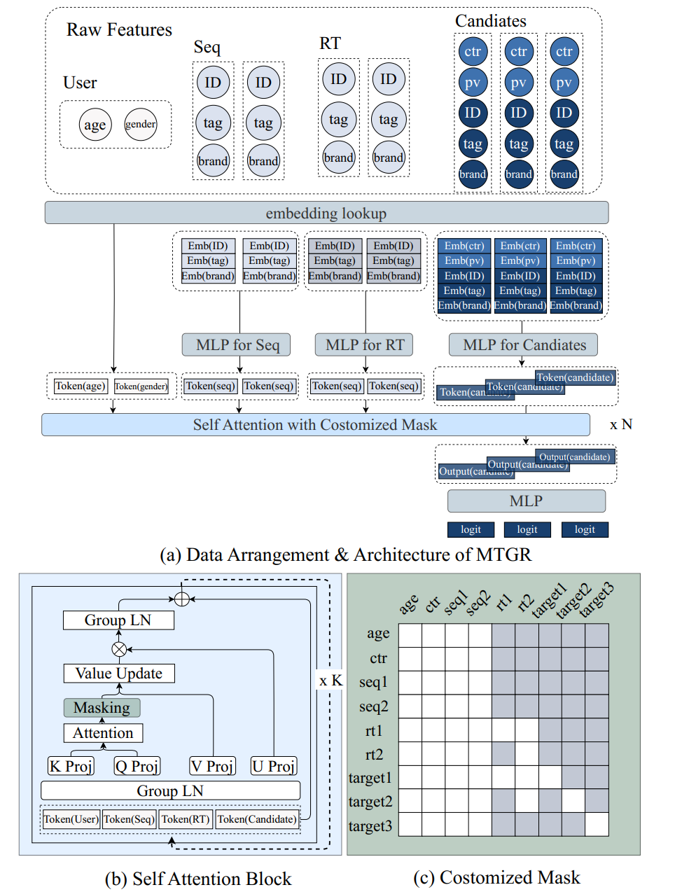
1. Adopt GR into the current production systemMTGR^[44] from Meituan is a great example that leverages the HSTU architecture, and keeps all features, including cross features, in the original deep learning recommendation model (DLRM) as shown in Figure 24.

2. Explore different model architectures for GR: The right architecture of GR is an open question under active research. HSTU architecture, a decoder-only structure with many customizations on transformer-like models coming from the use case insights and trial-and-errors, works best for Meta's workload. However, as we will describe in more details in later case studies, LinkedIn's LiGR47 found that standard transformer model architecture works better than the HSTU for their workload and Kuaishou's OneRec^[45] adopts an encoder-decoder architecture for a unified model to perform retrieval and ranking in one stage.

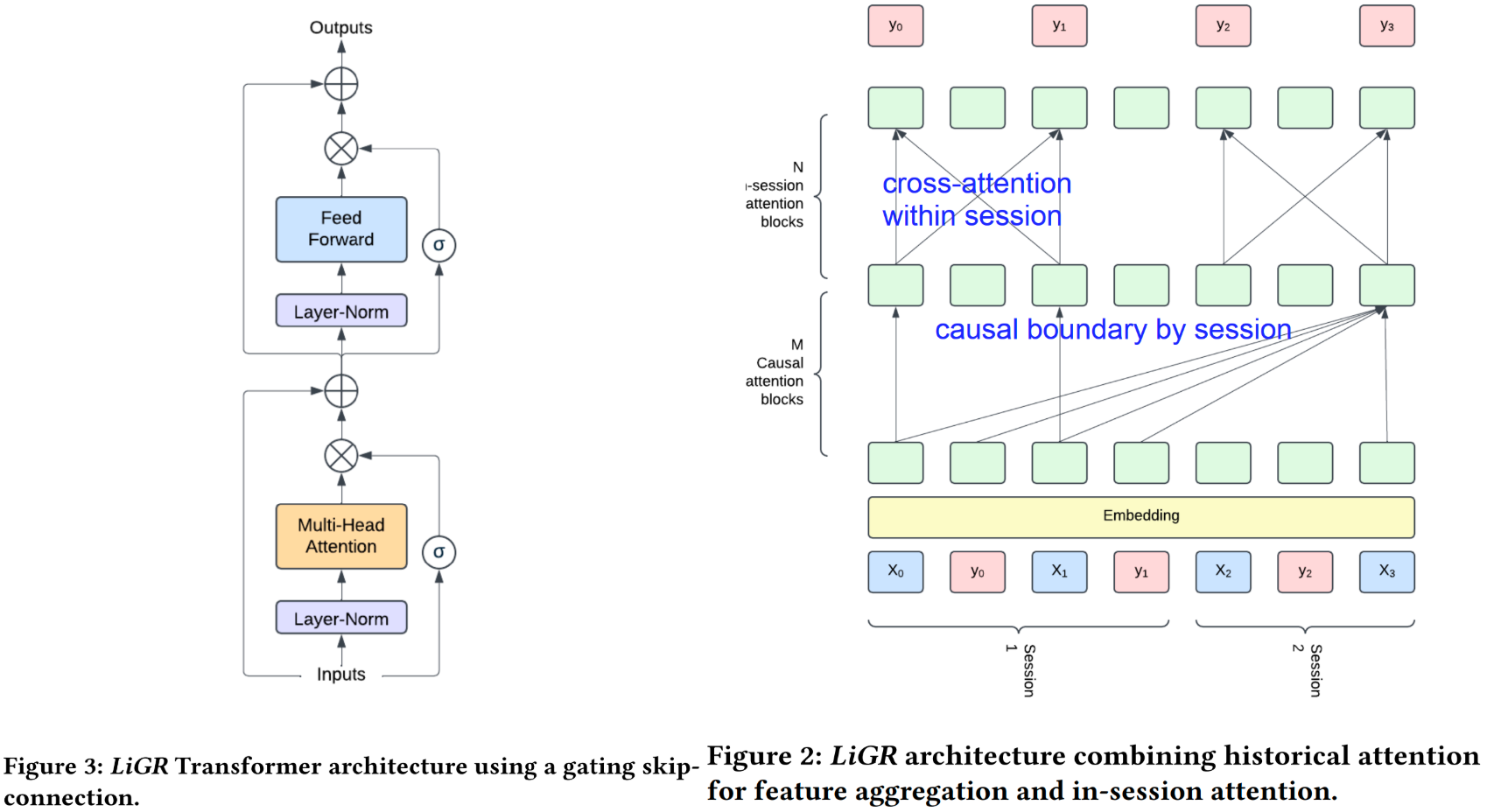
   • Case Study: LinkedIn's LiGR^[46]: Similarly, LiGR uses a fully sequential approach to perform recommendation tasks. Specifically, the model input is a member’s interaction history $X_0, X_1, \dots , X_n$, where each interaction $X_i$ represents one token. An input token $X_i$ is itself a concatenation of multiple embedding features which represent entities such as the item, the creator of the item, or content embeddings. The model output is a sequence $y_0, y_1, \dots , y_n$, which is the sequence of actions (click, like, comment, share, etc.) corresponding to the inputs. For example, $y_i$ would be a multi-hot vector representing all the actions that were taken on item $i$ by the member.

   For model architecture, as shown in Figure 25, LiGR introduces a modified transformer architecture that incorporates learned gated normalization and simultaneous set-wise attention to user history and ranked items. It also supports the concept of session with cross-attention within a session and ensuring causal boundary between sessions. This architecture enables several breakthrough achievements, including: (1) outperforming the prior state-of-the-art system using only 7 features (compared to hundreds in prior system), (2) validation of the scaling law for ranking systems, showing improved performance with larger models, more training data, and longer context sequences, and (3) simultaneous joint scoring of items in a set-wise manner, leading to automated improvements in diversity. To enable efficient, production-grade serving of large ranking models, we describe techniques to scale inference effectively using single-pass processing of user history and set-wise attention.

Performance wise, both GR from Meta and LiGR from LinkedIn have achieved significantly better performance than existing DLRM systems. Meta demonstrates that HSTU scales better than transformer in its use cases, while LiGR shows that the gated transformer achieves better performance and scales better with compute than HSTU. These somewhat contradicting results show that the right model for GR is an open question. The data for different use cases, the effort that each team spent on respective models, etc. could all impact the final conclusion. This shows that GR is still in early development and the field needs more experiments/results to converge the model architecture that is the most efficient and better attests the scaling law. The converged architecture will likely be another manifest of the bitter lesson in the future.

• Case Study: Kuaishou's OneRec (Towards Unification)^{[hou2024onerec@]}: This model embodies the vision of a single, unified model to cover both retrieval and ranking stages in one step as depicted in Figure 26.

More details in Figure 27 shows that it uses an encoder-decoder architecture with Mixture of Expert (MoE) at decoder stage and a session-wise generation approach to generate an entire slate of items at once. The iterative preference alignment (IPA) process further improves the quality of generation with direct preference optimization (DPO).

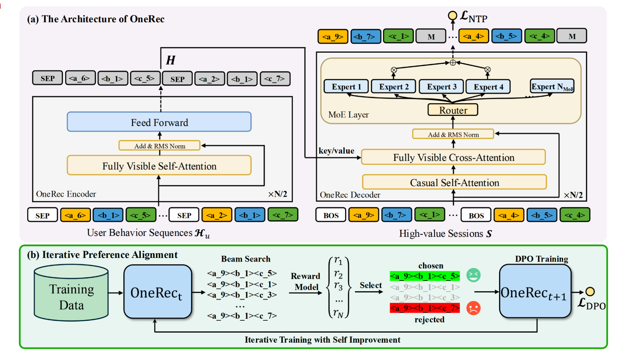
Crucially, its best performance relies on a discriminative reward model for preference alignment, indicating that for the foreseeable future, the most successful systems will likely be hybrids that combine a generative proposal network with a discriminative preference model.

• Case Study: Pinterest's PinRec (Generative Retrieval)^[47]: PinRec applies a generative model specifically to the retrieval stage. It is a sequential recommendation system and leverages a causal transformer decoder model architecture. The work developed two techniques to improve model performance: outcome-conditioned generation and multi-token generation.

1. Outcome-conditioned generation

This technique paves the way for multi-objective generation. At high-level, it is a budget-based auxiliary conditioning scheme that determines which outcome to use to condition the generation process based on its desirability represented by the budget. During the training process, the outcome is simply the next action; during inference, the outcome actions are used to condition generation based on the budget distribution, either deterministically or stochastically allocate a fixed number of items for each action during generation.

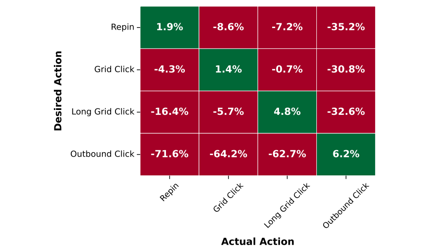
For simplicity, Figure 28 summarizes the offline evaluation with conditions across actions (repin, grid click, long grid click, and outbound click) when the budget is entirely allocated to one action at a time.

When matching outcome conditioning, consistent recall lifts are observed for all four actions, ranging from 1.9% for repin to 6.2% for outbound click. On the flip side, when the true action does not correspond to the desired action, recall decreases compared to an unconditioned baseline, indicating that conditioning achieves the desired result of producing outcome-specific representations.

2. Multi-token generation

One principal assumption in the next token objective is that there is strict ordering between the elements of the sequence. However, that reasoning is not necessarily applicable to item recommendation platforms, where a user may engage with a list of items in an arbitrary order within a session. The absence of strict ordering in sequential user engagement motivates the multi-token generation. Assume there exists a timestamp window of size $\Delta$ within which user activity is roughly time-equivalent (their order within that window is not significant). To incorporate the time-equivalent window size $\Delta$, the paper proposes a windowed multi-token objective. That is, for any future timestep window of size $\Delta$ starting at current timestamp, all items that are engaged within that window are targets for our prediction task. Intuitively, the generation problem becomes: can we sequentially predict any future items based on the set of items until now that users will engage within the time window $\Delta$ in the future. This problem is not only more aligned with the properties of user interactions, but also allows for significantly reduced serving latency since multiple items can be predicted at the same time.

• Case Study: Netflix FM for Personalized Recommendation50: Similarly, the work is inspired by the NLP trend of moving away from numerous small, specialized models towards a single, large language model that can perform a variety of tasks either directly or with minimal fine-tuning. Two critical insights guided the design of foundation model in Netflix:

1. A Data-Centric Approach: Shifting focus from model-centric strategies, which heavily rely on feature engineering, to a data-centric one. This approach prioritizes the accumulation of large-scale, high-quality data and, where feasible, aims for end-to-end learning.

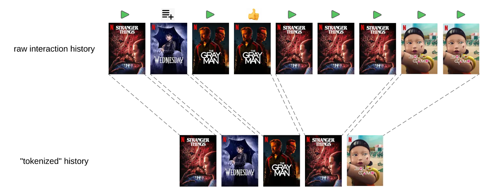
To leverage the user engagement data efficiently, Tokenizing User Interactions is proposed to deal with the fact that not all raw user actions contribute equality to understanding preferences Figure 29. Tokenization helps define what constitutes a meaningful “token” in a sequence. Drawing an analogy to Byte Pair Encoding (BPE) in NLP, we can think of tokenization as merging adjacent actions to form new, higher-level tokens. However, unlike language tokenization, creating these new tokens requires careful consideration of what information to retain. For instance, the total watch duration might need to be summed or engagement types aggregated to preserve critical details.

This tradeoff between granular data and sequence compression is akin to the balance in LLMs between vocabulary size and context window. In Netflix's case, the goal is to balance the length of interaction history against the level of detail retained in individual tokens. Overly lossy tokenization risks losing valuable signals, while too granular a sequence can exceed practical limits on processing time and memory.

Even with the tokenization, interaction histories from active users can span thousands of events, exceeding the capacity of transformer models with standard self attention layers. In recommendation systems, context windows during inference are often limited to hundreds of events — not due to model capability but because these services typically require millisecond-level latency. This constraint is more stringent than what is typical in LLM applications, where longer inference times (seconds) are more tolerable.

To address this during training, we implement two key solutions:

Sparse Attention Mechanisms: By leveraging sparse attention techniques such as low-rank compression, the model can extend its context window to several hundred events while maintaining computational efficiency. This enables it to process more extensive interaction histories and derive richer insights into long-term preferences.

Sliding Window Sampling: During training, we sample overlapping windows of interactions from the full sequence. This ensures the model is exposed to different segments of the user’s history over multiple epochs, allowing it to learn from the entire sequence without requiring an impractically large context window.

At inference time, when multi-step decoding is needed, we can deploy KV caching to efficiently reuse past computations and maintain low latency.

2. Leveraging Semi-Supervised Learning: The next-token prediction objective in LLMs has proven remarkably effective. It enables large-scale semi-supervised learning using unlabeled data while also equipping the model with a surprisingly deep understanding of world knowledge. The work adopted the autoregressive next-token prediction objective, similar to GPT. This strategy effectively leverages the vast scale of unlabeled user interaction data. Two key modifications have been tried on model objective and architecture:
   a. Multi-token prediction to deal with unequal token importance: During the pretraining phase of typical LLMs, such as GPT, every target token is generally treated with equal weight. In contrast, in our model, not all user interactions are of equal importance. For instance, a 5-minute trailer play should not carry the same weight as a 2-hour full movie watch. A greater challenge arises when trying to align long-term user satisfaction with specific interactions and recommendations. To address this, we can adopt a multi-token prediction objective during training, where the model predicts the next n tokens at each step instead of a single token. This approach encourages the model to capture longer-term dependencies and avoid myopic predictions focused solely on immediate next events.
   b. Auxiliary prediction objective to regularize overfitting: We can use multiple fields in our input data as auxiliary prediction objectives in addition to predicting the next item ID, which remains the primary target. For example, we can derive genres from the items in the original sequence and use this genre sequence as an auxiliary target. This approach serves several purposes: it acts as a regularizer to reduce overfitting on noisy item ID predictions, provides additional insights into user intentions or long-term genre preferences, and, when structured hierarchically, can improve the accuracy of predicting the target item ID. By first predicting auxiliary targets, such as genre or original language, the model effectively narrows down the candidate list, simplifying subsequent item ID prediction.

The resulting foundation model performance scales with the model size (compute) and has proven very effective in various downstream applications from direct use as a predictive model to generate user and entity embeddings for other applications, and can be fine-tuned for specific canvases. Overall, it achieves the goal of moving from multiple specialized models to a more comprehensive system and marks an exciting development in the field of personalized recommendation systems.

Agentic Paradigm #

The agentic paradigm is the most forward-looking application of FMs in recommendation. In this vision, the FM acts as the "brain" of an autonomous agent that can reason, plan, and interact with users and tools to fulfill complex goals. This moves beyond simple recommendation to a more holistic form of user assistance and the synergy between FMs and reinforcement learning.

• The Agentic Framework: An agentic recommender is characterized by its autonomy and its core components: a memory module to retain user history, a planning module to decompose complex requests into steps, and an action module to execute those steps, often by using external tools (like a search engine or a database). This allows the agent to dynamically adapt to user needs and evolving contexts.

  • Case Study: RecMind^[48] This LLM-powered agent provides zero-shot personalized recommendations by leveraging external knowledge and tools as illustrated in Figure. RecMind uses a "Self-Inspiring" planning algorithm where the LLM reflects on previously explored reasoning paths to make better decisions. It can use a database tool to query for specific user or item attributes and a search tool to access real-time information, allowing it to generate highly contextual and well-explained recommendations without being explicitly trained on the task.

  

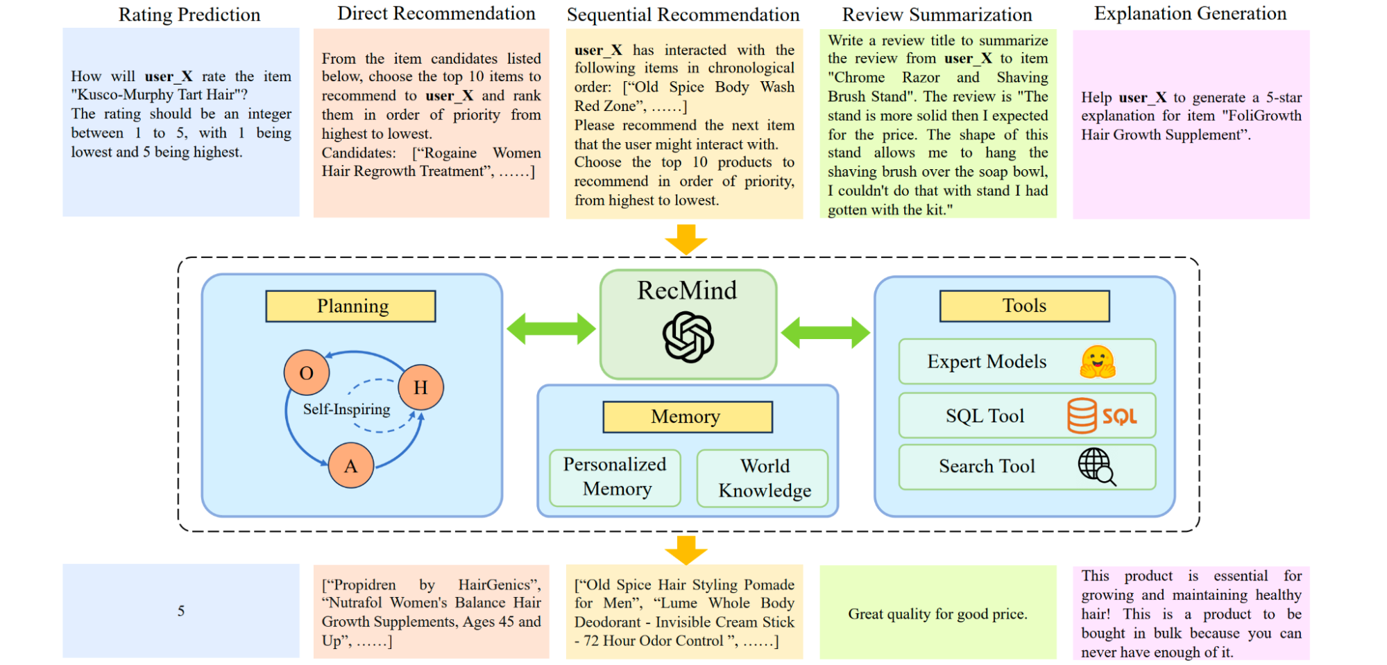
  • Case Study: Multi-Agent Simulation (Agent4Rec)^[49] This framework explores the use of a large number of LLM-powered agents to simulate realistic user interactions in a movie recommendation environment (Figure). Each of the 1,000 agents embodies unique social traits and preferences, allowing researchers to test new algorithms and understand user behavior at scale without needing real user studies. This highlights the agentic paradigm's role in creating sophisticated evaluation environments.

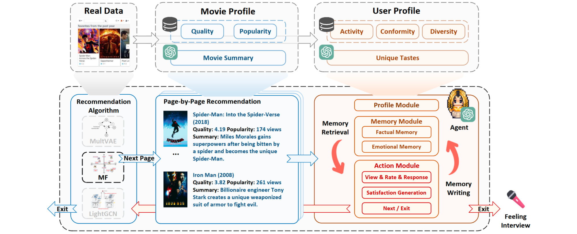
• The Symbiosis of FMs and Reinforcement Learning: The relationship between FMs and RL is a two-way street: FMs are solving some of RL's oldest and hardest problems, while RL is becoming essential for aligning the most advanced FMs.
  • FMs Solving RL's Core Challenges:
    • The Action Space Problem: A long-standing barrier to applying RL in slate recommendation is the combinatorial explosion of possible slates. The SlateQ solution in the Deep Learning era reduces the action space with some practical assumptions and only chooses the highest ranked slate in a category as a tradeoff. The GeMS^[50] framework offers an elegant solution by using a generative model (a VAE) to learn a continuous, low-dimensional latent space for slates (Figure 32). The RL agent then learns to act in this simple latent space, and the VAE's decoder translates its actions back into a full slate of items, making the problem tractable.

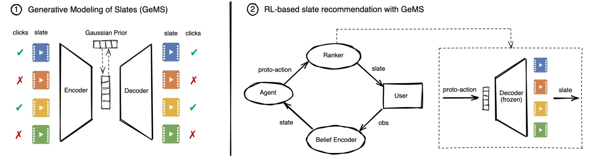
• The Offline Training Problem: The primary reason full RL deployments are rare is the risk of "distribution shift" when a policy trained on static logs is deployed online. A potential solution is the use of LLMs as high-fidelity user simulators. Frameworks like SimUSER^[51] prompt an LLM with a user profile and history, enabling it to generate realistic, human-like reactions to an RL agent's recommendations (Figure 33). This creates a safe and scalable "sandbox" for training and evaluating RL policies offline, dramatically accelerating the development of systems that can optimize for long-term user value.

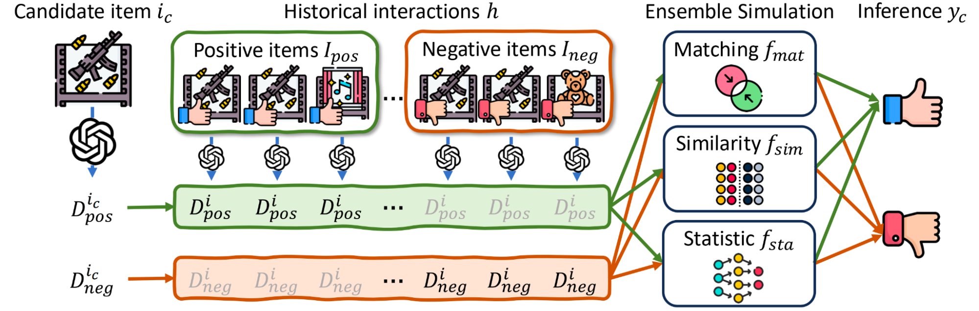
• RL Aligning FMs and Improving Recommendation:
  • Reinforcement Learning from Human/AI Feedback (RLHF/RLAIF): This technique is essential for aligning generative models with nuanced human preferences. First, a reward model is trained on human (or AI) feedback comparing different model outputs. Then, this reward model is used to provide a dense reward signal to fine-tune the generative model's policy using RL algorithms like Proximate Policy Optimization (PPO)^[52] and other recent variants like Group Relative Policy Optimization (GRPO)^[53]. This is particularly critical for conversational recommenders, where the goal is to optimize for user satisfaction over multi-turn dialogues. It's out of scope to expand on this topic and this book by N. Lambert^[54] has summarized RLHF really well and the author has done a good job updating the book to closely follow the development of the field.
  • Rec-R1: Bridging LLM and RecSys via RL^[55]. Unlike other case studies above that build foundation models from scratch, or prompting and supervised finetuning LLMs to improve RecSys, Rec-R1 improves the RecSys performance with a closed feedback loop between LLMs and RecSys leveraging reinforcement learning. As depicted in Figure 34, under Rec-R1, the LLMs treats the RecSys as a block-box and directly trains the LLM policy based on the feedback from the RecSys. The feedback reward signals are common metrics like NDVG@k and Recall@k. The GRPO algorithm is used to optimize the policy to significantly reduce memory consumption during training while maintaining competitive performance as compared to traditional algorithms such as PPO.

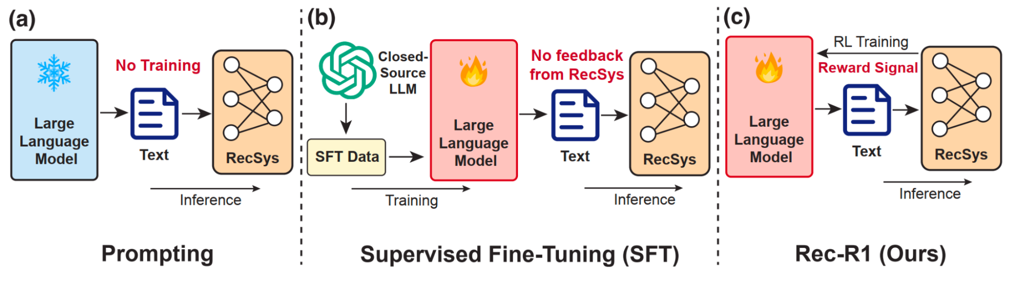
Here is the detailed problem formulation. Rec-R1 begins by modeling how LLMs are integrated into RecSys. In this general setup, the LLM receives an input $s \in S$, which may represent a user query, behavioral history, or contextual information. The LLM then generates a textual output $a \in A$, such as a rewritten query, an enriched item description, or a synthesized user profile. This output is consumed by a downstream recommendation model, which produces a performance-based evaluation $f(a|s) \in R$, such as NDCG, Recall, or any task-specific metric. The behavior of the LLM is governed by a conditional generation policy $\pi_{\theta}(a|s)$ where $\theta$ denotes the parameters of the generative LLM. The objective is to find a policy that maximizes expected recommendation performance:

Here, $p(s)$ denotes the empirical distribution over recommendation-relevant inputs provided to the LLM.

Rec-R1 conducted experiments in two representative tasks for RecSys: product search and sequential recommendation, and achieved encouraging results on both tasks as summarized in Table 2 and 3.

Table 2: Performance comparison of different methods on complex product search (Amazon-C4) tasks. We report the NDCG@100 scores. The best performance score is denoted in bold, with the second and third best underlined. The numbers in gray indicate the improvement of REC-R1 over their corresponding base retrievers (BM25 or BLAIR).

As shown in Table 2, Rec-R1 achieves the best performance across all four domains and retriever architectures, demonstrating strong generalization beyond the training distribution. This cross-domain evaluation highlights Rec-R1’s ability to generalize from training on one set of product categories to effectively handling unseen categories during testing. Moreover, prompting-based query rewriting using frozen LLMs (e.g., GPT-4o or Qwen-Instruct) either yields negligible improvement or even degrades performance—particularly on dense retrievers.

Table 3: Performance comparison of different methods on the sequential recommendation task on Amazon Beauty dataset. We report the Recall@k (R) and NDCG@k (N) scores. The best performance score is denoted in bold. The numbers in gray indicate the absolute improvement of REC-R1 over the initialized policy, i.e., Qwen-2.5-3B-Instruct.

For the sequential recommendation task, the evaluations are done with two test-time settings: (1) Transductive setting: All candidate items in the test sequence (both history and target) have appeared in the training set; (2) Inductive setting: None of the test-time items are seen during training.

Table 3 summarizes the performance under both transductive and inductive settings. The prompting-based baselines using frozen LLMs (e.g., GPT-4o and Qwen-2.5-3B-Instruct) perform poorly across the board—highlighting the difficulty of this task for generic LLMs without adaptation. However, when trained under the Rec-R1 framework, the finetuned Qwen-2.5-3B-Instruct model exhibits significant performance gains, especially in the inductive setting. For instance, in Recall@10 and NDCG@50, Rec-R1 improves upon its initialized policy by +4.20 and +2.64 points respectively. Moreover, Rec-R1 outperforms strong sequential baselines like UniSRec in the inductive setting, demonstrating its superiority in cold-start or unseen-item scenarios.

In the transductive setting, Rec-R1 remains competitive but lags behind specialized models. This is not surprising, as traditional sequential recommendation methods are explicitly trained on large-scale user-item sequences and directly model sequential dependencies. In contrast, Rec-R1 leverages LLMs to generate natural language queries about the user’s next likely purchase—relying on their strength in reasoning and generalization. However, next-item prediction based solely on interaction history is often not a task that lends itself to explicit reasoning in language space. The relationship between past and future items may be weak or non-causal, making it inherently difficult for LLMs to perform this task effectively, and models trained on these use-item sequences have advantages with the memorization effect or even overfitting.

The paper also checked how well each method (SFE or Rec-R1) can preserve the general-purpose capabilities of the underlying language model. Figure 35 summarizes three models across six tasks spanning different axes of generalization: ESCI (recommendation), MMLU (factual knowledge), IFEval (instruction following), GSM8K (math reasoning), and two coding benchmarks: MBPP and HumanEval. On ESCI, SFT yields improvements over the base model, while Rec-R1 achieves substantially higher gains—without relying on GPT-4o-generated data. On MMLU, all models—including Rec-R1 —achieve comparable accuracy. This suggests that neither SFT nor REC-R1 compromises the model’s general knowledge.

However, striking differences emerge on IFEval. Here, SFT suffers a dramatic performance drop—losing over 27 points—while Rec-R1 not only avoids degradation but actually improves slightly over the original model. This highlights a key advantage of our Rec-R1: by optimizing directly for task-specific performance without overriding the model’s generative distribution via next token prediction, Rec-R1 preserves instruction-following capabilities more effectively. A similar trend happens on GSM8K, where Rec-R1 improves upon the initialized model while SFT lags far behind. In contrast, both SFT and Rec-R1 maintain strong performance on coding tasks like MBPP and HumanEval. This is likely because our SFT data involved JSON-style outputs to facilitate answer extraction, which do not interfere with the model’s code generation ability. These results highlight the promise of Rec-R1 as a new paradigm for LLM adaptation—one that enables strong task-specific improvements without compromising general capabilities.

Overall, Rec-R1 demonstrates how RL bridges LLMs with RecSys through direct feedback. It achieves strong performance across tasks and retrievers while preserving general-purpose capabilities, offering a scalable alternative to prompting and SFT. It is a really promising general approach to optimize RecSys performance, especially when there is no access to change the RecSys internals.

Uncharted Territory: Open Questions and Challenges #

Despite the rapid progress, the generative paradigm raises fundamental questions and surfaces significant operational challenges that will shape the future of the field. Some of them are touched above, and here are a list to put them together with some rough thoughts:

• Is this the "ChatGPT Moment" for RecSys? There are compelling arguments that we are at a similar inflection point. The first major work that attests to scaling laws in RecSys at Meta—showing that model quality improves as a predictable power-law of the compute resource—is powerful evidence. This suggests that, as in NLP, simply scaling up models and data could lead to transformative capabilities. The potential to unify disparate tasks like retrieval, ranking, and explanation into a single foundation model represents a true paradigm shift. However, the analogy is not perfect. Language possesses a universal grammar that a model can learn. User behavior, in contrast, is often highly idiosyncratic and domain-specific. Furthermore, many of the most successful generative systems, like Kuaishou's OneRec, still rely on a discriminative reward model—which looks very much like a traditional ranker—to achieve their best performance, suggesting a purely generative approach may not yet be sufficient.
• Is generative recommender a good architecture for tasks beyond sequential recommendation? The current wave of generative recommenders has overwhelmingly focused on sequential recommendation—predicting the next item a user will interact with. This formulation is a natural fit for the auto-regressive nature of LLMs. However, it is less clear how this paradigm applies to other important recommendation tasks. For example, how does a generative model handle non-sequential problems like "basket completion" or "session-based recommendation" where user identity is unavailable? Moreover, many recommendation scenarios are heavily driven by immediate context (e.g., time of day, location) rather than a long historical sequence. Critical aspects like explainability, fairness, and controllability are also open areas of research; while generative models can produce explanations, ensuring they are faithful, factual, and unbiased is a major challenge.
• The Role of GR in Search Systems? Intuitively, search can be viewed as a special case of recommendation, explicitly conditioned on a user's query. This makes it a natural domain for generative models that can take a query as a prompt and directly generate relevant items (or semantic IDs for the items as discussed before). The primary challenge, however, is grounding. A search system must be factually accurate. The tendency of LLMs to hallucinate is a far greater risk in a search context than in a more exploratory recommendation context. Therefore, integrating generative models into search will likely rely heavily on Retrieval-Augmented Generation (RAG) architectures and robust fact-checking to ensure the generated results are both relevant and trustworthy.
• Model Robustness and Scalability: While FMs show great promise, ensuring their robustness in real-world, high-stakes environments is critical. They can be sensitive to input phrasing and require massive computational resources for both training and real-time inference, posing significant cost and latency challenges.
• Explainability and Trust: Generative models can produce fluent explanations, but ensuring these explanations are faithful to the model's internal reasoning and not just plausible-sounding "hallucinations" is a major hurdle. Building user trust requires a new level of transparency that is still an active area of research.
• Bias and Fairness: FMs are trained on internet data (unless trained from scratch with user engagement data like in some work above), which can contain and amplify societal biases. A generative recommender might produce biased explanations or recommendations that reinforce stereotypes. Auditing and mitigating these biases is significantly more complex in an open-ended generative model than in a traditional ranker with a fixed output space.
• Evaluation in the Generative Era: Traditional offline metrics like NDCG or AUC are insufficient for evaluating generative systems. They cannot measure the quality, coherence, or factuality of a generated explanation, nor can they detect hallucinations. A holistic evaluation framework is needed that assesses not just the relevance of the recommended items but also the safety, helpfulness, and truthfulness of the entire generative output, a significant and active area of research.

Summary: The Bitter Lesson and the Path Forward #

The evolutionary path of recommender systems provides a powerful, domain-specific illustration of Rich Sutton's "The Bitter Lesson". The history of recommendation algorithms, from the intuitive heuristics of the classical era to the foundation models of today, is a quintessential case study of this principle in action.

The journey began with methods that relied heavily on human intuition. The deep learning revolution was the first major turn of the screw for the bitter lesson, as general-purpose learning architectures began to systematically outperform systems built on manual feature engineering.

The current generative age represents the lesson's latest expression. The vision of a foundation model for recommendation is a bet on a maximally general-purpose method. By tokenizing the world of items and users into a unified "language" and applying a general sequence modeling architecture, this approach seeks to learn the fundamental "grammar" of user behavior entirely from data and computation. It is a direct move away from building in what we think we know, and towards building systems that can discover knowledge for themselves.

The path forward is therefore paved with both immense opportunity and significant challenges. The future of recommendation is likely to be defined by these unified, generative, and increasingly agentic architectures. The traditional lines separating retrieval and ranking, and even search and recommendation, are already beginning to blur. The most critical challenges are no longer purely algorithmic. Instead, they are systemic: building the next-generation infrastructure capable of training and serving these behemoth models efficiently, and developing the robust operational discipline required to manage their complexity, mitigate their novel risks like hallucination and bias, and ensure they are deployed responsibly and effectively. The bitter lesson teaches us that scale is the most powerful lever we have; the next decade of recommender systems will be defined by our ability to harness it.

References #