Understand Reasoning Engine: RL Infrastructure for LLMs, From Algorithms to Production
Abstract. The development of reasoning-capable LLMs has expanded the frontier of AI infrastructure beyond pre-training at scale, introducing Reinforcement Learning as a complementary and increasingly critical post-training dimension. This post traces the evolution of this new dimension through three paradigms—RLHF, RLVR, and Agentic RL—then dives into the systems architecture that makes RL training work at scale. Using SkyRL as a detailed case study, we run four head-to-head experiments on GSM8K comparing rule-based rewards vs. LLM-as-a-Judge rewards and synchronous vs. asynchronous training, revealing interesting differences in learning dynamics, throughput, and GPU cost. We conclude with a survey of open-source RL frameworks and a look at the frontier challenges ahead.
1. The Three Waves of RL in LLM Development #
The landscape of LLM development has expanded beyond pre-training compute to a multi-stage pipeline, including pre-training, mid-training, and post-training, and each contributes distinct capabilities. While pre-training continues to scale well and remains the foundation of model capability, a new and complementary scaling dimension has emerged: Reinforcement Learning for reasoning and alignment. Models such as DeepSeek-R1 and the OpenAI o-series demonstrate that RL-based post-training can unlock reasoning capabilities (chain-of-thought, self-correction, tool use) that pre-training and Supervised Fine-Tuning (SFT) alone struggle to produce. The Reinforcement Fine-Tuning (RFT) demands its own specialized infrastructure and optimization process, which is the focus of this post.
Post-training itself began with SFT which trains base models on curated instruction-response pairs to produce helpful assistants. SFT remains the foundation: it teaches models to follow instructions, adopt a conversational format, and produce coherent outputs. But SFT has an inherent ceiling—the model can only be as good as its training data, learning to imitate rather than to reason. RL breaks through this ceiling by optimizing for outcomes rather than imitation, allowing models to discover novel solution strategies that may not exist in any training corpus.
We can trace the evolution of RL in LLM development through three distinct waves, each building on the last.
Wave 1: RLHF — Aligning Models to Human Preferences #
The first wave of RL applied to LLMs was Reinforcement Learning from Human Feedback (RLHF), pioneered by InstructGPT[1] and later powering ChatGPT. Building on top of an SFT checkpoint, the recipe added:
- Reward Model Training: Train a separate neural network on human preference comparisons (which response is better?) to produce a scalar reward signal.
- RL Optimization: Use PPO (Proximal Policy Optimization)[2] to maximize the reward model's score, with a KL-divergence penalty to prevent the policy from drifting too far from the SFT checkpoint.
PPO follows the Actor-Critic paradigm: the Policy (Actor) generates text, while a Value Model (Critic) estimates expected future rewards to reduce variance in gradient estimation. The per-token reward is formulated as:
where is the reward model score and the KL term prevents "reward hacking"—gaming the reward model without genuinely improving quality.
The infrastructure cost was steep. Training PPO requires four models in GPU memory simultaneously: the Policy, the Value Model (often as large as the Policy), the Reference Model, and the Reward Model. This effectively quadrupled the memory footprint compared to standard SFT. (For a deeper dive into the PPO algorithm and its evolution, see our companion post From PPO to GRPO[3].)
Wave 2: RLVR — Reinforcement Learning with Verifiable Rewards #
The second wave arrived with a critical insight: for tasks with objectively verifiable answers, you don't need a neural reward model at all. DeepSeek-R1[4] demonstrated that RL with rule-based verification—checking whether a math answer is correct or code passes unit tests—could bootstrap genuine reasoning capabilities from scratch, including the emergent "aha moment" where models spontaneously develop chain-of-thought reasoning.
This paradigm shift was enabled by a new algorithm: Group Relative Policy Optimization (GRPO), introduced in DeepSeekMath[5]. GRPO eliminates the Critic model entirely. Instead of learning a value function, it estimates the baseline from group statistics:
- For each prompt, generate a group of outputs (e.g., ).
- Score each output with a verifiable reward function (binary: correct or not).
- Compute the advantage as the normalized deviation from the group mean:
This simple change has profound infrastructure consequences:
| Aspect | PPO (Wave 1) | GRPO (Wave 2) |
|---|---|---|
| Models in memory | 4 (Policy + Critic + Ref + Reward) | 1–2 (Policy + optional Ref) |
| Compute bottleneck | Balanced (train ≈ generate) | Inference-heavy (generate samples/prompt) |
| Reward source | Neural reward model (subjective) | Verifiable function (deterministic) |
| Best for | Alignment, subjective tasks | Math, code, verifiable reasoning |
The shift to GRPO moves the bottleneck firmly to the inference phase: generating 64 samples per prompt requires a high-throughput inference engine (vLLM, SGLang), and the training system must efficiently interleave generation and optimization.
Wave 3: Agentic RL — Learning to Use Tools #
The third and current wave extends RL beyond single-turn text generation to multi-turn, tool-using agents. Models learn not just to reason internally, but to interact with external tools—search engines, code interpreters, databases, web browsers—across extended trajectories.
This wave introduces new infrastructure challenges:
- Variable-length trajectories: Episodes may span dozens of tool calls, unlike the single generate-then-score loop of RLVR.
- Heterogeneous compute: Tool execution (CPU-bound, network-bound) must be interleaved with token generation (GPU-bound) without starving the accelerators.
- Complex reward signals: Rewards may come at the end of a long trajectory, requiring credit assignment across many steps.
Frameworks like SkyRL-Agent address this by abstracting tools as composable actions and using asynchronous dispatchers to maximize GPU utilization during tool-waiting periods.
The Paradigm Stack #
These three waves of RL are cumulative, not replacements, and they all build on the SFT foundation. A modern reasoning model pipeline typically involves:
Pre-training → SFT → RLVR (math/code) → RLHF (alignment) → Agentic RL (tool use)
               ───    ──────────────────────────────────────────────────────────────
               Foundation              Three waves of RL
The infrastructure must support all of these stages, ideally within a single framework. This requirement for generality is what drives the architectural decisions we examine next.
2. Anatomy of Reinforcement Training System for LLMs #
RL training for LLMs is fundamentally different from supervised training. While SFT involves a simple forward-backward loop on static data, RL requires a dynamic feedback loop where the model generates data, the environment scores it, and the optimizer updates the model. All in an online, iterative cycle.
2.1 The Core Components #
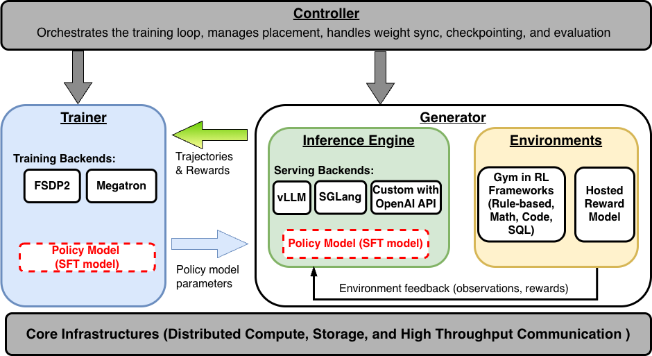
A modern Reinforcement Finetuning system for LLMs consists of four tightly-coupled components:
Trainer: Performs policy optimization using the configured RL algorithm (PPO, GRPO, RLOO, etc.). The trainer manages distributed gradient computation (with frameworks such as Fully Sharded Data Parallelism (FSDP) or Megatron), optimizer state, and model checkpointing. In GRPO, the trainer receives a batch of (prompt, response, reward) tuples, computes group-normalized advantages, and performs clipped policy gradient updates.
Generator: Produces trajectories by combining inference and environment execution. For each prompt in a batch, the generator:
- Sends the prompt to the Inference Engine to produce completions.
- Passes each completion to the Environment to compute rewards.
- Returns the scored trajectories to the trainer.
Inference Engine: A high-throughput LLM serving engine (typically vLLM or SGLang) that generates text from the current policy weights. The engine must support:
- Weight synchronization: After each training step, the updated policy weights must be synced to the inference engine.
- Sleep/wake modes: When colocated with training on the same GPU, the engine must release memory during training and reclaim it during generation.
- Batched generation: Processing multiple prompts × multiple samples per prompt efficiently.
Environment / Reward: Scores each generated response. This is where the critical design decision of rule-based vs. LLM-as-a-Judge lives—a choice that we'll explore in depth in Section 3.
These components can be colocated on the same GPU(s) (time-sharing via sleep/wake) or disaggregated across dedicated GPUs to enable pipeline parallelism. We'll see both configurations in action in Section 3.
2.2 Weight Synchronization #
After each training step, the policy model's updated weights must be propagated to the inference engine(s). This is a critical bottleneck, especially in disaggregated setups. Common strategies include:
- NCCL/CUDA IPC (colocated): Direct GPU-to-GPU memory copy on the same node. Near-instant, but requires shared GPU access.
- NCCL Broadcast (disaggregated): High-bandwidth collective communication across nodes. Fast on InfiniBand/RDMA, slower on commodity Ethernet.
- Checkpoint-and-load: The trainer saves weights to shared storage; the inference engine reloads them. Simple but slow—useful as a fallback or for heterogeneous hardware.
For a 0.5B parameter model in bfloat16, the weight tensor is ~1 GB. With NCCL broadcast over 10 Gbps Ethernet, this takes ~1 second—a fixed overhead that represents 8% of a 13-second training step but only 3% of a 31-second step with LLM-as-a-Judge (as we'll see in Section 3).
2.3 The RL Training Loop in Practice #
Putting it all together, a single GRPO training step looks like this:
1. SAMPLE prompts from the dataset (batch_size prompts)
2. GENERATE G responses per prompt via the Inference Engine
3. SCORE each response via the Environment (rule-based or LLM judge)
4. COMPUTE group-normalized advantages: Â_i = (r_i - mean(r)) / std(r)
5. COMPUTE policy loss with clipped importance sampling (PPO-style)
6. UPDATE policy weights via optimizer step
7. SYNC weights to inference engine(s)
8. Repeat
The relative cost of each phase depends heavily on the model size, group size , generation length, and—critically—the reward mechanism.
2.4 Framework Landscape #
The ecosystem of RL frameworks for LLMs has diversified rapidly. Each framework makes different trade-offs along the axes of performance, modularity, and accessibility.
| Framework | Origin | Architecture | Best For | Key Differentiator |
|---|---|---|---|---|
| SkyRL | Berkeley Sky Lab + Anyscale | Ray + vLLM/SGLang, modular Trainer/Generator/Env | Agentic RL, research prototyping | Full-stack modularity (skyrl-train + skyrl-gym + skyrl-agent); easy environment development |
| veRL | ByteDance | HybridFlow (single-controller), 3D-HybridEngine | Large-scale production training | Zero-redundancy weight sharing between train/inference modes; extreme scaling |
| OpenRLHF | Community | Ray + vLLM + DeepSpeed | Maximum throughput at scale | Clean "token-in-token-out" abstraction; Ring Attention for long context; proven production stability |
| TRL | Hugging Face | Transformers + PEFT | Quick experimentation, single-GPU | Lowest barrier to entry; tight HF ecosystem integration; GRPO support |
| NeMo-RL | NVIDIA | NeMo + Megatron | Frontier model training | 5D parallelism; FP8 pipeline; optimized for H100/B200 clusters |
| Unsloth | Community | Custom Triton kernels | Consumer GPU training | 90% VRAM reduction via manual backprop; GRPO on a single 48GB GPU for 70B models |
How should we choose? The decision depends on where you sit on the stack:
- Inventing new reasoning processes (novel environments, tools, agent architectures) → SkyRL or TRL for their modularity and low barrier to environment development.
- Scaling known recipes to hundreds of GPUs → veRL, OpenRLHF, or NeMo-RL for their systems-level optimizations.
- Democratizing access on limited hardware → Unsloth for its kernel-level memory efficiency.
- Training MoE models at the frontier → NeMo-RL for its Megatron integration and numerical stability features.
In this post, we use SkyRL[6] for our case study because of its clean separation between the training framework (skyrl-train) and the environment library (skyrl-gym). This modularity allowed us to implement and compare two different reward mechanisms—rule-based and LLM-as-a-Judge—without modifying any core training code.
3. Case Study: GSM8K on SkyRL with Rule-Based vs. LLM-as-a-Judge #
To make the concepts above concrete, we ran four head-to-head experiments training a Qwen2.5-0.5B-Instruct policy model on GSM8K[7] (grade-school math, 7,473 training problems) using GRPO, varying two independent axes:
- Reward mechanism: Rule-based (extract
####answer, compare to gold) vs. LLM-as-a-Judge (a Qwen2.5-1.5B-Instruct model evaluates correctness). - Training mode: Synchronous (generation and training are sequential) vs. Asynchronous (generation runs one step ahead of training, overlapping with the previous step's optimization).
All experiments use identical hyperparameters (learning rate, batch size, group size, etc.) and the same GRPO algorithm. This 2×2 design isolates the effects of reward mechanism and training mode on infrastructure cost, throughput, and learning dynamics. Settings for all experiments are available in the SkyRL repository.
3.1 Experimental Setup #
Common hyperparameters (shared across all four runs):
| Parameter | Value |
|---|---|
| Policy model | Qwen2.5-0.5B-Instruct |
| Algorithm | GRPO (group size ) |
| Train batch size | 16 |
| Learning rate | 1e-6 |
| KL loss | Disabled |
| Max generate length | 1024 tokens |
| Weight sync | NCCL broadcast |
Why is KL loss disabled? (click to expand)
KL divergence penalty is the classic regularizer in RLHF (Equation 1), designed to prevent the policy from drifting too far from the reference model and gaming a learned reward model. In GRPO on verifiable tasks, we disable it for several reinforcing reasons:
- No neural reward model → nothing to hack. With rule-based rewards, the answer is either correct or not—there's no soft neural judge to exploit, so the primary motivation for KL regularization disappears.
- The clipped objective already constrains updates. GRPO uses PPO-style clipped importance ratios, which bound the policy update to . This serves the same stabilizing role as KL, making both together overly conservative.
- KL suppresses exploration. For reasoning tasks, the model needs to discover qualitatively different solution strategies. The KL penalty anchors the policy to the reference model, which can prevent emergent reasoning patterns—the DeepSeek-R1 paper found that removing KL improved reasoning capability.
- Memory savings. Disabling KL eliminates the need to keep a reference model in memory, dropping from 2 models to 1—critical for fitting on a single L4 GPU.
Per-configuration details:
| Configuration | Reward Model | GPUs | Placement |
|---|---|---|---|
| Sync + Rule-Based | — (string matching) | 1 × L4 | Colocated (policy + inference on 1 GPU) |
| Sync + LLM Judge | Qwen2.5-1.5B-Instruct | 2 × L4 | Colocated policy + disaggregated reward |
| Async + Rule-Based | — (string matching) | 2 × L4 | Disaggregated (1 train + 1 inference) |
| Async + LLM Judge | Qwen2.5-1.5B-Instruct | 3 × L4 | Disaggregated (1 train + 1 inference + 1 reward) |
GPU Layouts:
Sync + Rule-Based (1 GPU):               Sync + LLM Judge (2 GPUs):
┌──────────────────┐                     ┌──────────────────┐  ┌──────────────────┐
│     L4 GPU       │                     │    L4 GPU 1      │  │    L4 GPU 2      │
│                  │                     │                  │  │                  │
│ Policy (0.5B)    │                     │ Policy (0.5B)    │  │ Reward (1.5B)    │
│ + vLLM Inference │                     │ + vLLM Inference │  │ Frozen vLLM      │
│ (colocated,      │                     │ (colocated,      │  │ (always active)  │
│  sleep/wake)     │                     │  sleep/wake)     │  │                  │
│                  │                     │                  │  │                  │
│ Reward: instant  │                     │ Reward: → GPU 2  │  │ ← scores here    │
│ (string match)   │                     │ (Ray actor call)  │  │                  │
└──────────────────┘                     └──────────────────┘  └──────────────────┘

Async + Rule-Based (2 GPUs):              Async + LLM Judge (3 GPUs):
┌──────────────────┐ ┌──────────────────┐ ┌──────────┐ ┌──────────┐ ┌──────────┐
│    L4 GPU 1      │ │    L4 GPU 2      │ │ L4 GPU 1 │ │ L4 GPU 2 │ │ L4 GPU 3 │
│                  │ │                  │ │          │ │          │ │          │
│  FSDP Policy     │ │ vLLM Inference   │ │  FSDP    │ │  vLLM    │ │ Reward   │
│  (training)      │ │ (generation)     │ │  Policy  │ │  Infer.  │ │  (1.5B)  │
│                  │ │                  │ │ (train)  │ │  (gen)   │ │  Frozen  │
│  ◄── weight sync ──►                 │ │  ◄──sync──►          │ │          │
└──────────────────┘ └──────────────────┘ └──────────┘ └──────────┘ └──────────┘
 Generate runs 1 step ahead of Train       Generate runs 1 step ahead of Train
In the synchronous configurations, generation and training are strictly sequential on the same GPU(s)—the inference engine sleeps during training and wakes for generation. In the asynchronous configurations, the generator runs one step ahead: while the trainer optimizes on batch , the inference engine is already generating batch . This overlap requires disaggregated placement (colocate_all=false), as the trainer and inference engine must run concurrently on separate GPUs.
The LLM-as-a-Judge configurations use a FrozenRewardInferenceClient—a subclass of SkyRL's InferenceEngineClient that creates vLLM engines without weight-sync capabilities (since the reward model never changes). The reward engine is exposed as a named Ray actor ("reward_inference_service"), and environments discover it automatically—no HTTP servers, no port conflicts, no stale subprocesses.
3.2 Throughput Comparison #
The table below shows mean per-step timing across all four configurations (averaged over the full run of each experiment):
| Metric | Sync Rule-Based | Sync LLM Judge | Async Rule-Based | Async LLM Judge |
|---|---|---|---|---|
| Generate | 10.7s | 18.0s | 11.3s | 20.3s |
| Policy train | 4.7s | 5.3s | 4.8s | 5.1s |
| Weight sync | 1.2s | 1.2s | 1.9s | 1.9s |
| Total step | 21.9s | 30.6s | 13.8s | 22.1s |
| GPUs | 1 | 2 | 2 | 3 |
| Throughput | 2.9 samples/s | 2.1 samples/s | 4.6 samples/s | 2.9 samples/s |
Several patterns emerge:
Reward mechanism is the dominant cost axis. Adding the LLM judge increases step time by ~40% in both sync and async modes (21.9→30.6s sync, 13.8→22.1s async). For each of the 64 generated responses per batch (16 prompts × 4 samples), the 1.5B reward model must generate a judgment of up to 512 tokens. This ~8–10s of reward inference per step is the fundamental cost of neural reward evaluation.
Async training provides consistent speedup. Async reduces step time by 37% for rule-based (21.9→13.8s) and 28% for LLM judge (30.6→22.1s). The overlap is effective because the ~5s policy training phase runs concurrently with the next batch's generation. The speedup is larger for rule-based because a higher fraction of the step time is train+sync (which gets overlapped), whereas the LLM judge bottleneck is in generation itself (which can't be overlapped).
Disaggregated weight sync is slightly more expensive. Weight sync increases from ~1.2s (colocated, CUDA IPC) to ~1.9s (disaggregated, NCCL broadcast over Ethernet)—a 0.7s overhead that is dwarfed by the overlap savings.
3.3 The Reward Trajectory Surprise #
The most striking finding isn't throughput—it's the learning dynamics. The reward trajectories reveal two distinct phenomena: the dramatic effect of reward mechanism, and the consistency of learning across training modes.
         ── Sync ──────────────    ── Async ─────────────
Step    Rule-Based  LLM Judge    Rule-Based  LLM Judge
  1      0.016       0.766        0.000       0.766
  5      0.031       0.859        0.016       0.859
 10      0.063       0.859        0.094       0.922
 15      0.047       0.859        0.063       0.797
 20      0.188       0.875        0.141       0.750
 25      0.203       0.891        0.281       0.906
 30      0.328       0.953        0.422       0.922
 35      0.328       0.953        0.328       0.922
 40      0.453       0.953        0.406       0.859
 45      0.484       0.938        0.594       0.969
 50      0.594       1.000        —           0.875
Two patterns jump out:
1. Reward mechanism dominates the starting point. At step 1, the LLM judge gives a reward of ~0.77 while the rule-based reward gives ~0.01. Same model, same prompts, same answers—but dramatically different scores.
2. Sync vs. async produces nearly identical learning curves. For each reward type, the sync and async trajectories track each other closely—despite the async trainer using weights that are one step stale. This validates that for GRPO with small learning rates (1e-6), the mild off-policy bias from async training is benign.
What explains the 50× gap in starting reward between the two reward mechanisms?
3.4 Analysis: What This Tells Us About Reward Design #
The gap reveals a fundamental difference in what each reward mechanism measures:
Rule-based reward measures format + correctness jointly. The gsm8k environment extracts the final answer using the regex #### (-?[0-9.,]+) and compares it to the gold answer. If the model solves the problem correctly but doesn't format the answer as #### 42, it receives a reward of zero. At step 1, Qwen2.5-0.5B-Instruct is a capable math model—it often produces the right answer—but it rarely formats it with the #### delimiter. The model must learn both mathematical reasoning and output formatting simultaneously.
LLM-as-a-Judge measures correctness only. The 1.5B judge model reads both the gold solution and the generated solution, understands the mathematical content, and can recognize a correct answer regardless of format. It doesn't care whether the answer says #### 42, The answer is 42, or 42. This format-agnostic evaluation means the model starts at a much higher reward because it already knows the math—it just hasn't learned the format.
This is a textbook illustration of reward shaping:
| Aspect | Rule-Based | LLM-as-Judge |
|---|---|---|
| What it rewards | Format compliance + correctness | Correctness only |
| Starting reward | Low (must learn format) | High (model already capable) |
| Learning signal | Teaches both reasoning and discipline | Teaches reasoning only |
| GRPO signal quality | Higher variance → richer gradient signal | Lower variance → weaker gradient signal |
| Reward hacking risk | Low (deterministic) | Higher (judge can be gamed) |
| Applicable to | Verifiable tasks only | Any task with a reference answer |
The counterintuitive insight: The rule-based reward's low starting point is actually a feature, not a bug. Because rewards start near zero with high variance across the group, GRPO gets a strong gradient signal—most samples score 0, and the rare correct+formatted sample scores 1, creating a clear learning direction. With the LLM judge, most samples already score ~0.8, so the normalized advantages are small and the gradient signal is weaker.
Reward inflation: comparing curves across reward functions is apples-to-oranges. The LLM judge's reward of 0.77 at step 1 doesn't mean the model is 77% accurate—it means the judge thinks it's correct 77% of the time. The model hasn't been updated at all! The gap reflects a difference in measurement leniency, not model capability. The judge gives credit for correct reasoning regardless of output format, inflating the reward relative to what the model can actually produce in a format-compliant way. To truly compare which reward mechanism teaches math faster, one would need to evaluate both on a held-out test set using a common metric (e.g., rule-based exact-match accuracy). The reward curves alone can't answer that question.
The cost-effectiveness question is surprisingly open. The LLM judge reaches high reward faster in wall-clock steps, but each step costs 2.8× more GPU-seconds (2 GPUs × 30.6s vs. 1 GPU × 21.9s). Rule-based rewards start slow but are cheap—and the strong gradient signal from high variance may produce more sample-efficient learning per GPU-hour. Whether total GPU-cost to reach a target test accuracy favors one approach over the other depends on the task, model size, and how much of the judge's leniency translates to genuine capability gains vs. reward inflation. For instance, if both approaches reach 80% test accuracy, but rule-based takes 100 steps on 1 GPU while LLM judge takes 40 steps on 2 GPUs, the rule-based approach is actually cheaper (100 × 21.9 = 2,190 GPU-seconds vs. 40 × 30.6 × 2 = 2,448 GPU-seconds). This is an empirical question that merits controlled study—and one that becomes increasingly important as policy models scale to 7B+ parameters, where the reward model must scale accordingly.
Reward hacking risk grows with training. The table above flags LLM-as-a-Judge as having higher reward hacking risk, but it's worth emphasizing why. A deterministic rule-based reward is unforgeable: the answer is either 42 or it isn't. An LLM judge, however, can be exploited—the policy may learn to produce outputs that look correct to the 1.5B judge but aren't actually right. Worse, this gap between judge reward and actual accuracy can widen as training progresses, because the policy is being optimized to please the judge, not to solve the math. This is precisely the reward hacking problem that the KL penalty in Equation 1 was designed to mitigate in RLHF—and it applies equally when using an LLM judge for RLVR tasks. Rule-based rewards sidestep this entirely.
3.5 When to Use Each Approach #
Use rule-based rewards when:
- The task has objectively verifiable answers (math, code, SQL)
- You want deterministic, reproducible training
- You want the model to learn specific output formatting
- GPU budget is limited (no reward model GPU needed)
Use LLM-as-a-Judge when:
- The task requires subjective evaluation (creative writing, summarization, relevance scoring)
- The evaluation criteria can't be captured by simple string matching
- You need format-agnostic evaluation during development
- The reward model can provide richer feedback than binary correct/incorrect
Use both (in sequence) when:
- You want to validate that your rule-based reward isn't too restrictive or too lenient
- You want to compare reward signal quality for a given task
- You're writing a blog post about RL infrastructure :)
3.6 Implementation Highlights #
A key advantage of SkyRL's modular architecture is that switching between reward mechanisms required zero changes to the training code. The only differences are:
- The environment class:
gsm8k(rule-based) vs.llm_as_a_judge_local(LLM judge) - The run script: Whether to start a reward inference service
The rule-based environment is 30 lines of Python:
class GSM8kEnv(BaseTextEnv):
    def __init__(self, env_config=None, extras={}):
        super().__init__()
        self.ground_truth = extras["reward_spec"]["ground_truth"]

    def step(self, action: str) -> BaseTextEnvStepOutput:
        reward = utils.compute_score(action, self.ground_truth)
        return BaseTextEnvStepOutput(
            observations=[], reward=reward, done=True, metadata={}
        )
The LLM-as-a-Judge environment calls a Ray actor wrapping a frozen vLLM engine:
class GSM8kLLMJudgeLocalEnv(BaseTextEnv):
    def __init__(self, env_config, extras={}):
        super().__init__()
        self.ground_truth = extras["reward_spec"]["ground_truth"]
        self._reward_service = ray.get_actor("reward_inference_service")

    def _get_reward(self, action: str) -> float:
        message = PROMPT + f"\nGOLD: {self.ground_truth}\nPREDICTED: {action}"
        reply = ray.get(self._reward_service.score.remote(
            [{"role": "user", "content": message}]
        ))
        match = re.search(r"Final\s*Score\s*[:=]\s*([01])", reply)
        return float(match.group(1)) if match else 0.0
The FrozenRewardInferenceClient that backs this service is a subclass of SkyRL's InferenceEngineClient that creates vLLM engines without weight-sync capabilities. It inherits load balancing and placement-group GPU scheduling from the base class, and adds score() / score_batch() methods for text-level reward evaluation. Scaling from 1 to N reward engines is a single config change (num_reward_engines=N).
3.7 Sync vs. Async: When Does Pipelining Pay Off? #
Our four experiments provide a controlled comparison of synchronous vs. asynchronous training. The key question: does overlapping generation and training justify the extra GPU?
Synchronous:   [Generate 10.7s]──[Train 4.7s]──[Sync 1.2s]──[Generate]──...
                                                              Total: 21.9s/step

Asynchronous:  [Generate 11.3s]──────[Generate 11.3s]──────[Generate]──...
                    ──[Train 4.8s]──[Sync 1.9s]──[Train]──...
                                                              Total: 13.8s/step
               (overlap saves ~8s/step)
The speedup depends on the overlap ratio—how much of the training+sync phase can be hidden behind the next generation:
| Configuration | Generate | Train+Sync | Overlap Potential | Actual Speedup | Extra GPUs |
|---|---|---|---|---|---|
| Rule-Based | 10.7s | 5.9s | 55% of step | 37% (21.9→13.8s) | +1 GPU |
| LLM Judge | 18.0s | 6.5s | 36% of step | 28% (30.6→22.1s) | +1 GPU |
The async speedup is larger for rule-based because training represents a bigger fraction of the total step time. With LLM judge, the generation phase (including reward scoring) dominates so much that the training phase is already a small slice—there's less to overlap.
Is the extra GPU worth it? For rule-based, async delivers 4.6 samples/s across 2 GPUs vs. 2.9 samples/s on 1 GPU—a 59% efficiency gain per GPU-hour. For LLM judge, async delivers 2.9 samples/s across 3 GPUs vs. 2.1 samples/s on 2 GPUs—a 38% efficiency loss per GPU-hour (but 38% higher absolute throughput, useful when wall-clock time matters more than GPU-hours).
The practical takeaway: Async training is most valuable when (a) generation and training have comparable costs, and (b) wall-clock time matters more than GPU efficiency. For inference-dominated workloads (large models, long sequences, LLM-as-Judge), the benefit is more nuanced—async still helps wall-clock time but at a GPU efficiency cost. Of course, we could allocate more resources to inference and training to increase throughput further, but that's out of scope for this post.
4. Exploration and Future Directions #
Our GSM8K experiments, while focused on a single task, expose several open challenges and directions for RL infrastructure at large.
4.1 Reward Model Scaling #
Our LLM-as-a-Judge used a 1.5B reward model to judge a 0.5B policy. In practice, reward models should be at least as capable as the policy being trained—otherwise the judge cannot distinguish good from bad responses. As policy models scale to 7B, 70B, and beyond, the reward model must scale accordingly, making the GPU cost of LLM-as-a-Judge increasingly significant.
Several approaches address this:
- Reward model distillation: Train a small, fast reward model from a large teacher.
- Reward caching: Cache reward scores for identical (prompt, response) pairs across epochs.
- Hybrid rewards: Use rule-based rewards for verifiable components and LLM judge only for subjective aspects.
4.2 Multi-Turn and Agentic RL #
Single-turn GRPO on GSM8K is the "Hello World" of RL for LLMs. The frontier is multi-turn agentic RL, where models learn to use tools, navigate environments, and solve tasks requiring dozens of interactions. This introduces challenges that our simple experiments don't capture:
- Credit assignment over long horizons: Which tool call in a 20-step trajectory was responsible for success?
- Environment latency: Waiting for web searches, code execution, or database queries creates GPU idle time.
- Context window management: Long trajectories consume context, requiring efficient attention mechanisms or context compression.
SkyRL's agent layer (skyrl-agent) addresses these through a tool-centric architecture where tool calls are first-class actions, and an asynchronous dispatcher that interleaves GPU-bound generation with CPU-bound tool execution.
4.3 Early Stopping and Compute Efficiency #
Our GSM8K experiments showed the model reaching high rewards within 50–100 steps. For harder datasets like DAPO-Math-17k or AIME competition problems, the reward curve would be slower, but the principle holds: most of the learning happens in the first fraction of training. Early stopping based on reward saturation—automatically halting when the rolling average reward plateaus—could save significant compute, especially during hyperparameter sweeps.
4.4 The Disaggregation of the RL Pipeline #
A clear trend across the framework ecosystem is the disaggregation of the RL pipeline into services:
- Inference as a Service: Frameworks increasingly treat generation as a remote procedure call to a high-performance engine (vLLM, SGLang), decoupled from the training loop.
- Reward as a Service: Our
FrozenRewardInferenceClientexemplifies this pattern—the reward model runs as a named Ray actor, discoverable by any environment on any node, with its own GPU allocation and lifecycle. - Training as a Service: The policy optimizer, with its FSDP sharding and gradient accumulation, operates independently and communicates via weight sync protocols.
This service-oriented architecture mirrors the broader trend in ML systems toward composable, independently scalable components—a far cry from the monolithic training scripts of the SFT era.
4.5 What's Next #
The RL infrastructure landscape is evolving rapidly. Key areas to watch:
- On-policy distillation: Combining RL exploration with knowledge distillation from stronger models.
- Unified SFT/RL engines: Systems like SkyRL-tx that provide a single engine for both supervised and reinforcement training, eliminating the need for separate pipelines.
- RL on MoE models: Expert routing decisions depend on batch composition and parallelism strategy, so the same tokens can be routed to different experts during rollout generation (inference engine) vs. training (training framework). This mismatch corrupts the log-probability estimates that PPO/GRPO rely on. Solutions like Rollout Routing Replay address this by saving routing decisions during generation and replaying them during the training forward pass.
Conclusion #
The "Reasoning Era" has forced a maturity upon RL infrastructure that didn't exist two years ago. We've moved past the initial phase of hacking PPO onto SFT trainers. Today's frameworks—SkyRL, veRL, OpenRLHF, TRL, NeMo-RL, Unsloth—represent a sophisticated diversification of tools, each optimized for a different point on the spectrum from accessibility to scalability.
Our four GSM8K experiments illustrate that even for a "simple" task, the choice of reward mechanism and training mode has cascading effects on infrastructure cost (1–3 GPUs), throughput (13.8–30.6s per step), and learning dynamics (format-strict vs. format-agnostic). Async training delivered 28–37% step-time improvements with negligible impact on learning curves, while LLM-as-a-Judge and rule-based rewards produced dramatically different reward trajectories from the same model. These are not just engineering details—they are design decisions that shape what the model learns and how efficiently it learns it.
For practitioners, the takeaways are:
- Start with rule-based rewards whenever possible. They're faster, cheaper, deterministic, and provide stronger gradient signals through higher reward variance.
- Use async training when wall-clock time matters. The extra GPU pays for itself with a 37% speedup for rule-based and 28% for LLM judge, with no measurable impact on learning quality.
- Reserve LLM-as-a-Judge for tasks that genuinely require subjective evaluation—and when you do, treat the reward model as a first-class infrastructure component with its own GPU budget, scaling strategy, and lifecycle management.
The future of AI reasoning will be built not only just on better algorithms, but also on the diverse and capable infrastructure layer that supports them.
References #
Citation #
If you found this useful, please cite this blog as:
Guanghua Shu and Non-linear AI. (Feb 2026). Understand Reasoning Engine: RL Infrastructure for LLMs, From Algorithms to Production. non-linear.ai. https://non-linear.ai/blog/rl-for-post-training/
or
@article{shu2026rlposttraining,
  title   = {Understand Reasoning Engine: RL Infrastructure for LLMs, From Algorithms to Production},
  author  = {{Guanghua Shu and Non-linear AI}},
  journal = {non-linear.ai},
  year    = {2026},
  month   = {Feb},
  url     = {https://non-linear.ai/blog/rl-for-post-training/}
}